Document feedback

Question document fragment

When a question document fragment contains a formula, it is displayed as a space.

Submission type

issue

It's a little complicated...

I'd like to ask someone.

PR

Just a small problem.

I can fix it online!

Please select the submission type

Problem type

Specifications and Common Mistakes

- Specifications and Common Mistakes:

- Misspellings or punctuation mistakes,incorrect formulas, abnormal display.

- Incorrect links, empty cells, or wrong formats.

- Chinese characters in English context.

- Minor inconsistencies between the UI and descriptions.

- Low writing fluency that does not affect understanding.

- Incorrect version numbers, including software package names and version numbers on the UI.

Usability

- Usability:

- Incorrect or missing key steps.

- Missing main function descriptions, keyword explanation, necessary prerequisites, or precautions.

- Ambiguous descriptions, unclear reference, or contradictory context.

- Unclear logic, such as missing classifications, items, and steps.

Correctness

- Correctness:

- Technical principles, function descriptions, supported platforms, parameter types, or exceptions inconsistent with that of software implementation.

- Incorrect schematic or architecture diagrams.

- Incorrect commands or command parameters.

- Incorrect code.

- Commands inconsistent with the functions.

- Wrong screenshots.

- Sample code running error, or running results inconsistent with the expectation.

Risk Warnings

- Risk Warnings:

- Lack of risk warnings for operations that may damage the system or important data.

Content Compliance

- Content Compliance:

- Contents that may violate applicable laws and regulations or geo-cultural context-sensitive words and expressions.

- Copyright infringement.

Please select the type of question

Problem description

Describe the bug so that we can quickly locate the problem.

Document feedback

PINNs for Kovasznay Flow

Problem Description

This tutorial demonstrates how to solve the Kovasznay flow problem using Physics-Informed Neural Networks (PINNs). Kovasznay flow is an exact solution of the Navier-Stokes (N-S) equations under certain conditions. Kovasznay flow satisfies the momentum equation and continuity equation of the N-S equations, and it also satisfies Dirichlet boundary conditions.

The velocity and pressure distribution of the Kovasznay flow can be represented by the following equations:

u = 1 - e^{λ x} \cos (2 π y),

v = \frac{λ}{2 π} e^{λ x} \sin (2 π x),

p = \frac{1}{2} (1 - e^{2 λ x})

Here, $λ = \frac{1}{2 ν} - \sqrt{\frac{1}{4 ν^{2}} + 4 π^{2}}$ .

We can use the Kovasznay flow as a benchmark solution to verify the accuracy and stability of the PINNs method.

Technical Pathway

The specific steps to solve this problem using MindSpore Flow are as follows:

Create the training dataset.
Build the model.
Set up the optimizer.
Define the constraints.
Train the model.
Evaluate the model.

[1]:

import time

from mindspore import context, nn, ops, jit
from mindflow import load_yaml_config
from mindflow.cell import FCSequential
from mindflow.loss import get_loss_metric
from mindspore import load_checkpoint, load_param_into_net, save_checkpoint

from src.dataset import create_dataset


context.set_context(mode=context.GRAPH_MODE, save_graphs=False, device_target="GPU")

# Load config
file_cfg = "kovasznay_cfg.yaml"
config = load_yaml_config(file_cfg)

Creating the Dataset

In this tutorial, we randomly sample the solution domain and boundary conditions to generate the training dataset and test dataset. The specific method can be found in src/dataset.py.

[2]:

ds_train = create_dataset(config)

Building the Model

In this example, we use a simple fully connected neural network with a depth of 4 layers. Each layer consists of 50 neurons, and the activation function used is tanh.

[3]:

model = FCSequential(
    in_channels=config["model"]["in_channels"],
    out_channels=config["model"]["out_channels"],
    layers=config["model"]["layers"],
    neurons=config["model"]["neurons"],
    residual=config["model"]["residual"],
    act="tanh",
)

[2]:

if config["load_ckpt"]:
    param_dict = load_checkpoint(config["load_ckpt_path"])
    load_param_into_net(model, param_dict)

params = model.trainable_params()
optimizer = nn.Adam(params, learning_rate=config["optimizer"]["initial_lr"])

Kovasznay Solver

The Kovasznay Solver consists of two parts: the Kovasznay flow equation and the boundary conditions.

The boundary conditions are set based on the reference solution mentioned above.

[4]:

import sympy
from sympy import Function, diff, symbols
from mindspore import numpy as ms_np
from mindflow import PDEWithLoss, sympy_to_mindspore
import math

class Kovasznay(PDEWithLoss):
    """Define the loss of the Kovasznay flow."""

    def __init__(self, model, re=20, loss_fn=nn.MSELoss()):
        """Initialize."""
        self.re = re
        self.nu = 1 / self.re
        self.l = 1 / (2 * self.nu) - math.sqrt(
            1 / (4 * self.nu**2) + 4 * math.pi**2
        )
        self.x, self.y = symbols("x y")
        self.u = Function("u")(self.x, self.y)
        self.v = Function("v")(self.x, self.y)
        self.p = Function("p")(self.x, self.y)
        self.in_vars = [self.x, self.y]
        self.out_vars = [self.u, self.v, self.p]
        super(Kovasznay, self).__init__(model, self.in_vars, self.out_vars)
        self.bc_nodes = sympy_to_mindspore(self.bc(), self.in_vars, self.out_vars)
        if isinstance(loss_fn, str):
            self.loss_fn = get_loss_metric(loss_fn)
        else:
            self.loss_fn = loss_fn

    def pde(self):
        """Define the gonvering equation."""
        u, v, p = self.out_vars
        u_x = diff(u, self.x)
        u_y = diff(u, self.y)
        v_x = diff(v, self.x)
        v_y = diff(v, self.y)
        p_x = diff(p, self.x)
        p_y = diff(p, self.y)
        u_xx = diff(u_x, self.x)
        u_yy = diff(u_y, self.y)
        v_xx = diff(v_x, self.x)
        v_yy = diff(v_y, self.y)
        momentum_x = u * u_x + v * u_y + p_x - (1 / self.re) * (u_xx + u_yy)
        momentum_y = u * v_x + v * v_y + p_y - (1 / self.re) * (v_xx + v_yy)
        continuty = u_x + v_y
        equations = {
            "momentum_x": momentum_x,
            "momentum_y": momentum_y,
            "continuty": continuty,
        }
        return equations

    def u_func(self):
        """Define the analytical solution."""
        u = 1 - sympy.exp(self.l * self.x) * sympy.cos(2 * sympy.pi * self.y)
        return u

    def v_func(self):
        """Define the analytical solution."""
        v = (
            self.l
            / (2 * sympy.pi)
            * sympy.exp(self.l * self.x)
            * sympy.sin(2 * sympy.pi * self.y)
        )
        return v

    def p_func(self):
        """Define the analytical solution."""
        p = 1 / 2 * (1 - sympy.exp(2 * self.l * self.x))
        return p

    def bc(self):
        """Define the boundary condition."""
        bc_u = self.u - self.u_func()
        bc_v = self.v - self.v_func()
        bc_p = self.p - self.p_func()
        bcs = {"u": bc_u, "v": bc_v, "p": bc_p}
        return bcs

    def get_loss(self, pde_data, bc_data):
        """Define the loss function."""
        pde_res = self.parse_node(self.pde_nodes, inputs=pde_data)
        pde_residual = ops.Concat(axis=1)(pde_res)
        pde_loss = self.loss_fn(pde_residual, ms_np.zeros_like(pde_residual))
        bc_res = self.parse_node(self.bc_nodes, inputs=bc_data)
        bc_residual = ops.Concat(axis=1)(bc_res)
        bc_loss = self.loss_fn(bc_residual, ms_np.zeros_like(bc_residual))
        return pde_loss + bc_loss


# Create the problem
problem = Kovasznay(model)

momentum_x: u(x, y)*Derivative(u(x, y), x) + v(x, y)*Derivative(u(x, y), y) + Derivative(p(x, y), x) - 0.05*Derivative(u(x, y), (x, 2)) - 0.05*Derivative(u(x, y), (y, 2))
    Item numbers of current derivative formula nodes: 5
momentum_y: u(x, y)*Derivative(v(x, y), x) + v(x, y)*Derivative(v(x, y), y) + Derivative(p(x, y), y) - 0.05*Derivative(v(x, y), (x, 2)) - 0.05*Derivative(v(x, y), (y, 2))
    Item numbers of current derivative formula nodes: 5
continuty: Derivative(u(x, y), x) + Derivative(v(x, y), y)
    Item numbers of current derivative formula nodes: 2
u: u(x, y) - 1 + exp(-1.81009812001397*x)*cos(2*pi*y)
    Item numbers of current derivative formula nodes: 3
v: v(x, y) + 0.905049060006983*exp(-1.81009812001397*x)*sin(2*pi*y)/pi
    Item numbers of current derivative formula nodes: 2
p: p(x, y) - 0.5 + 0.5*exp(-3.62019624002793*x)
    Item numbers of current derivative formula nodes: 3

Model Training

Using MindSpore version >= 2.0.0, we can train neural networks using the functional programming paradigm.

[6]:

def train(config):
    grad_fn = ops.value_and_grad(
        problem.get_loss, None, optimizer.parameters, has_aux=False
    )

    @jit
    def train_step(pde_data, bc_data):
        loss, grads = grad_fn(pde_data, bc_data)
        loss = ops.depend(loss, optimizer(grads))
        return loss

    def train_epoch(model, dataset, i_epoch):
        model.set_train()
        n_step = dataset.get_dataset_size()
        for i_step, (pde_data, bc_data) in enumerate(dataset):
            local_time_beg = time.time()
            loss = train_step(pde_data, bc_data)

            if i_step % 50 == 0:
                print(
                    "\repoch: {}, loss: {:>f}, time elapsed: {:.1f}ms [{}/{}]".format(
                        i_epoch,
                        float(loss),
                        (time.time() - local_time_beg) * 1000,
                        i_step + 1,
                        n_step,
                    )
                )

    for i_epoch in range(config["epochs"]):
        train_epoch(model, ds_train, i_epoch)

    if config["save_ckpt"]:
        save_checkpoint(model, config["save_ckpt_path"])

[7]:

time_beg = time.time()
train(config)
print("End-to-End total time: {} s".format(time.time() - time_beg))

epoch: 0, loss: 0.239163, time elapsed: 12387.2ms [1/125]
epoch: 0, loss: 0.087055, time elapsed: 112.7ms [51/125]
epoch: 0, loss: 0.086475, time elapsed: 101.6ms [101/125]
epoch: 1, loss: 0.085488, time elapsed: 100.8ms [1/125]
epoch: 1, loss: 0.087387, time elapsed: 102.1ms [51/125]
epoch: 1, loss: 0.083520, time elapsed: 47.9ms [101/125]
epoch: 2, loss: 0.083846, time elapsed: 98.7ms [1/125]
epoch: 2, loss: 0.082749, time elapsed: 44.8ms [51/125]
epoch: 2, loss: 0.081391, time elapsed: 98.0ms [101/125]
epoch: 3, loss: 0.081744, time elapsed: 50.7ms [1/125]
epoch: 3, loss: 0.080608, time elapsed: 49.5ms [51/125]
epoch: 3, loss: 0.082139, time elapsed: 45.9ms [101/125]
epoch: 4, loss: 0.080847, time elapsed: 98.0ms [1/125]
epoch: 4, loss: 0.083495, time elapsed: 94.8ms [51/125]
epoch: 4, loss: 0.083020, time elapsed: 100.2ms [101/125]
epoch: 5, loss: 0.079421, time elapsed: 104.1ms [1/125]
epoch: 5, loss: 0.062890, time elapsed: 46.3ms [51/125]
epoch: 5, loss: 0.018953, time elapsed: 45.8ms [101/125]
epoch: 6, loss: 0.012071, time elapsed: 47.8ms [1/125]
epoch: 6, loss: 0.007686, time elapsed: 46.1ms [51/125]
epoch: 6, loss: 0.006134, time elapsed: 45.0ms [101/125]
epoch: 7, loss: 0.005750, time elapsed: 52.1ms [1/125]
epoch: 7, loss: 0.004908, time elapsed: 45.4ms [51/125]
epoch: 7, loss: 0.003643, time elapsed: 51.7ms [101/125]
epoch: 8, loss: 0.002799, time elapsed: 106.3ms [1/125]
epoch: 8, loss: 0.002110, time elapsed: 48.1ms [51/125]
epoch: 8, loss: 0.001503, time elapsed: 96.3ms [101/125]
epoch: 9, loss: 0.001195, time elapsed: 102.4ms [1/125]
epoch: 9, loss: 0.000700, time elapsed: 101.1ms [51/125]
epoch: 9, loss: 0.000478, time elapsed: 48.1ms [101/125]
epoch: 10, loss: 0.000392, time elapsed: 98.8ms [1/125]
epoch: 10, loss: 0.000315, time elapsed: 101.7ms [51/125]
epoch: 10, loss: 0.000236, time elapsed: 74.3ms [101/125]
epoch: 11, loss: 0.000218, time elapsed: 101.4ms [1/125]
epoch: 11, loss: 0.000184, time elapsed: 95.5ms [51/125]
epoch: 11, loss: 0.000171, time elapsed: 101.4ms [101/125]
epoch: 12, loss: 0.000145, time elapsed: 98.7ms [1/125]
epoch: 12, loss: 0.000144, time elapsed: 63.7ms [51/125]
epoch: 12, loss: 0.000126, time elapsed: 53.3ms [101/125]
epoch: 13, loss: 0.000111, time elapsed: 104.6ms [1/125]
epoch: 13, loss: 0.000109, time elapsed: 101.1ms [51/125]
epoch: 13, loss: 0.000090, time elapsed: 96.6ms [101/125]
epoch: 14, loss: 0.000094, time elapsed: 53.5ms [1/125]
epoch: 14, loss: 0.000079, time elapsed: 100.6ms [51/125]
epoch: 14, loss: 0.000070, time elapsed: 99.3ms [101/125]
epoch: 15, loss: 0.000193, time elapsed: 105.3ms [1/125]
epoch: 15, loss: 0.000066, time elapsed: 87.6ms [51/125]
epoch: 15, loss: 0.000118, time elapsed: 56.9ms [101/125]
epoch: 16, loss: 0.000074, time elapsed: 106.2ms [1/125]
epoch: 16, loss: 0.000054, time elapsed: 102.3ms [51/125]
epoch: 16, loss: 0.000065, time elapsed: 46.3ms [101/125]
epoch: 17, loss: 0.000050, time elapsed: 104.9ms [1/125]
epoch: 17, loss: 0.000056, time elapsed: 100.7ms [51/125]
epoch: 17, loss: 0.000045, time elapsed: 96.5ms [101/125]
epoch: 18, loss: 0.000043, time elapsed: 98.0ms [1/125]
epoch: 18, loss: 0.000043, time elapsed: 48.0ms [51/125]
epoch: 18, loss: 0.000050, time elapsed: 99.1ms [101/125]
epoch: 19, loss: 0.000038, time elapsed: 97.1ms [1/125]
epoch: 19, loss: 0.000051, time elapsed: 93.8ms [51/125]
epoch: 19, loss: 0.000044, time elapsed: 101.2ms [101/125]
End-to-End total time: 236.90019822120667 s

[8]:

from src import visual, calculate_l2_error

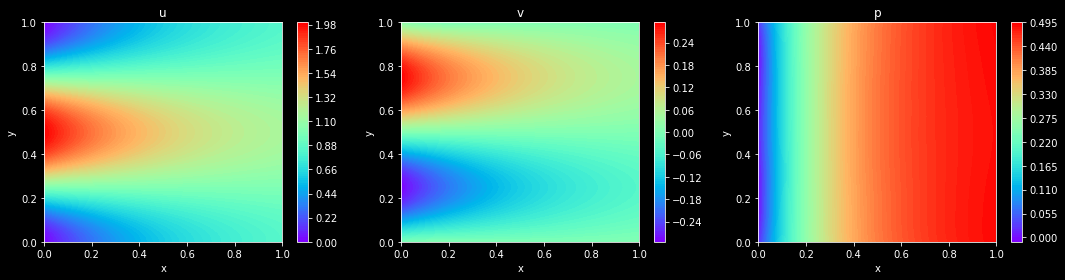
Model Prediction and Visualization

[9]:

visual(model, config, resolution=config["visual_resolution"])

../_images/physics_driven_kovasznay_15_0.png

Model Evaluation

[10]:

n_samps = 10000  # Number of test samples
ds_test = create_dataset(config, n_samps)
calculate_l2_error(problem, model, ds_test)

u: 1 - exp(-1.81009812001397*x)*cos(2*pi*y)
    Item numbers of current derivative formula nodes: 2
v: -0.905049060006983*exp(-1.81009812001397*x)*sin(2*pi*y)/pi
    Item numbers of current derivative formula nodes: 1
p: 0.5 - 0.5*exp(-3.62019624002793*x)
    Item numbers of current derivative formula nodes: 2
Relative L2 error on domain: 0.003131713718175888
Relative L2 error on boundary: 0.0069109550677239895