Document feedback

Question document fragment

When a question document fragment contains a formula, it is displayed as a space.

Submission type

issue

It's a little complicated...

I'd like to ask someone.

Please select the submission type

Problem type

Specifications and Common Mistakes

- Specifications and Common Mistakes:

- Misspellings or punctuation mistakes,incorrect formulas, abnormal display.

- Incorrect links, empty cells, or wrong formats.

- Chinese characters in English context.

- Minor inconsistencies between the UI and descriptions.

- Low writing fluency that does not affect understanding.

- Incorrect version numbers, including software package names and version numbers on the UI.

Usability

- Usability:

- Incorrect or missing key steps.

- Missing main function descriptions, keyword explanation, necessary prerequisites, or precautions.

- Ambiguous descriptions, unclear reference, or contradictory context.

- Unclear logic, such as missing classifications, items, and steps.

Correctness

- Correctness:

- Technical principles, function descriptions, supported platforms, parameter types, or exceptions inconsistent with that of software implementation.

- Incorrect schematic or architecture diagrams.

- Incorrect commands or command parameters.

- Incorrect code.

- Commands inconsistent with the functions.

- Wrong screenshots.

- Sample code running error, or running results inconsistent with the expectation.

Risk Warnings

- Risk Warnings:

- Lack of risk warnings for operations that may damage the system or important data.

Content Compliance

- Content Compliance:

- Contents that may violate applicable laws and regulations or geo-cultural context-sensitive words and expressions.

- Copyright infringement.

Please select the type of question

Problem description

Describe the bug so that we can quickly locate the problem.

Submit

Document feedback

FNO for 2D Navier-Stokes

  

Overview

Computational fluid dynamics is one of the most important techniques in the field of fluid mechanics in the 21st century. The flow analysis, prediction and control can be realized by solving the governing equations of fluid mechanics by numerical method. Traditional finite element method (FEM) and finite difference method (FDM) are inefficient because of the complex simulation process (physical modeling, meshing, numerical discretization, iterative solution, etc.) and high computing costs. Therefore, it is necessary to improve the efficiency of fluid simulation with AI.

Machine learning methods provide a new paradigm for scientific computing by providing a fast solver similar to traditional methods. Classical neural networks learn mappings between finite dimensional spaces and can only learn solutions related to specific discretizations. Different from traditional neural networks, Fourier Neural Operator (FNO) is a new deep learning architecture that can learn mappings between infinite-dimensional function spaces. It directly learns mappings from arbitrary function parameters to solutions to solve a class of partial differential equations. Therefore, it has a stronger generalization capability. More information can be found in the paper, Fourier Neural Operator for Parametric Partial Differential Equations.

This tutorial describes how to solve the Navier-Stokes equation using Fourier neural operator.

Navier-Stokes equation

Navier-Stokes equation is a classical equation in computational fluid dynamics. It is a set of partial differential equations describing the conservation of fluid momentum, called N-S equation for short. Its vorticity form in two-dimensional incompressible flows is as follows:

$${\partial }_{t}w(x,t)+u(x,t)\cdot \mathrm{\nabla }w(x,t)=\nu \mathrm{\Delta }w(x,t)+f(x),x\in (0,1{)}^2,t\in (0,T]$$

$$\mathrm{\nabla }\cdot u(x,t)=0,x\in (0,1{)}^2,t\in [0,T]$$

$$w(x,0)=w_0(x),x\in (0,1{)}^2$$

where $u$ is the velocity field, $w=\mathrm{\nabla }\times u$ is the vorticity, $w_0(x)$ is the initial vorticity, $\nu$ is the viscosity coefficient, $f(x)$ is the forcing function.

Problem Description

We aim to solve two-dimensional incompressible N-S equation by learning the operator mapping from each time step to the next time step:

$$w_t\mapsto w(\cdot ,t+1)$$

Technology Path

MindFlow solves the problem as follows:

1. Training Dataset Construction.

2. Model Construction.

3. Optimizer and Loss Function.

4. Define Solver.

5. Define Callback.

6. Model Training.

Fourier Neural Operator

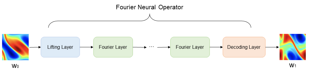
The following figure shows the architecture of the Fourier Neural Operator model. In the figure, $w_0(x)$ represents the initial vorticity. The input vector is lifted to higher dimension channel space by the lifting layer. Then the mapping result is used as the input of the Fourier layer to perform nonlinear transformation of the frequency domain information. Finally, the decoding layer maps the transformation result to the final prediction result $w_1(x)$.

The Fourier Neural Operator consists of the lifting Layer, Fourier Layers, and the decoding Layer.

Fourier layers: Start from input V. On top: apply the Fourier transform $\mathcal{F}$; a linear transform R on the lower Fourier modes and filters out the higher modes; then apply the inverse Fourier transform ${\mathcal{F}}^{-1}$. On the bottom: apply a local linear transform W. Finally, the Fourier Layer output vector is obtained through the activation function.

import os
import numpy as np

from mindspore import nn, context, Tensor, set_seed
from mindspore import DynamicLossScaleManager, LossMonitor, TimeMonitor, CheckpointConfig, ModelCheckpoint

The following src pacakage can be downloaded in applications/data_driven/navier_stokes/src.

from mindflow import FNO2D, RelativeRMSELoss, Solver, load_yaml_config, get_warmup_cosine_annealing_lr

from src import PredictCallback, create_training_dataset

set_seed(0)
np.random.seed(0)

context.set_context(mode=context.GRAPH_MODE, save_graphs=False, device_target='GPU')

config = load_yaml_config('navier_stokes_2d.yaml')
data_params = config["data"]
model_params = config["model"]
optimizer_params = config["optimizer"]
callback_params = config["callback"]

Training Dataset Construction

Download the training and test dataset: data_driven/navier_stokes/dataset .

In this case, training data sets and test data sets are generated according to Zongyi Li’s data set in Fourier Neural Operator for Parametric Partial Differential Equations . The settings are as follows:

The initial condition $w_0(x)$ is generated according to periodic boundary conditions:

$$w_0\sim \mu ,\mu =\mathcal{N}(0,7^{3/2}(-\mathrm{\Delta }+49I{)}^{-2.5})$$

The forcing function is defined as:

$$f(x)=0.1(\sin \left(2\pi (x_1+x_2)\right)+\cos (2\pi (x_1+x_2)))$$

We use a time-step of 1e-4 for the Crank–Nicolson scheme in the data-generated process where we record the solution every t = 1 time units. All data are generated on a 256 × 256 grid and are downsampled to 64 × 64. In this case, the viscosity coefficient $\nu =1e-5$, the number of samples in the training set is 19000, and the number of samples in the test set is 3800.

train_dataset = create_training_dataset(data_params, input_resolution=model_params["input_resolution"], shuffle=True)
test_input = np.load(os.path.join(data_params["path"], "test/inputs.npy"))
test_label = np.load(os.path.join(data_params["path"], "test/label.npy"))

Data preparation finished

Model Construction

The network is composed of 1 lifting layer, multiple Fourier layers and 1 decoding layer:

• The Lifting layer corresponds to the FNO2D.fc0 in the case, and maps the output data $x$ to the high dimension;

• Multi-layer Fourier Layer corresponds to the FNO2D.fno_seq in the case. Discrete Fourier transform is used to realize the conversion between time domain and frequency domain;

• The Decoding layer corresponds to FNO2D.fc1 and FNO2D.fc2 in the case to obtain the final predictive value.

model = FNO2D(in_channels=model_params["in_channels"],
              out_channels=model_params["out_channels"],
              resolution=model_params["input_resolution"],
              modes=model_params["modes"],
              channels=model_params["width"],
              depth=model_params["depth"]
              )

Optimizer and Loss Function

steps_per_epoch = train_dataset.get_dataset_size()
lr = get_warmup_cosine_annealing_lr(lr_init=optimizer_params["initial_lr"],
                                    last_epoch=optimizer_params["train_epochs"],
                                    steps_per_epoch=steps_per_epoch,
                                    warmup_epochs=optimizer_params["warmup_epochs"])

optimizer = nn.Adam(model.trainable_params(), learning_rate=Tensor(lr))
loss_scale = DynamicLossScaleManager()

# prepare loss function
loss_fn = RelativeRMSELoss()

Define Solver

Solver class is the interface for model training and evaluation. Given the optimizer, network model, loss function, loss scaling strategy, etc. the solver object can be defined easily. Parameters of optimizer_params and model_params can be modified in configuration file.

solver = Solver(model,
                optimizer=optimizer,
                loss_scale_manager=loss_scale,
                loss_fn=loss_fn,
                )

Define Callback

summary_dir = os.path.join(callback_params["summary_dir"], 'FNO2D')
print(summary_dir)
pred_cb = PredictCallback(model=model,
                          inputs=test_input,
                          label=test_label,
                          config=callback_params,
                          summary_dir=summary_dir)

ckpt_config = CheckpointConfig(save_checkpoint_steps=callback_params["save_checkpoint_steps"] * steps_per_epoch,
                               keep_checkpoint_max=callback_params["keep_checkpoint_max"])
ckpt_dir = os.path.join(summary_dir, "ckpt")
ckpt_cb = ModelCheckpoint(prefix=model_params["name"],
                          directory=ckpt_dir,
                          config=ckpt_config)

./FNO2D
check test dataset shape: (200, 19, 64, 64, 1), (200, 19, 64, 64, 1)

Model Training

Invoke the Solver interface for model training and callback interface for evaluation.

solver.train(epoch=optimizer_params["train_epochs"],
             train_dataset=train_dataset,
             callbacks=[LossMonitor(), TimeMonitor(), pred_cb, ckpt_cb],
             dataset_sink_mode=True)

epoch: 1 step: 1000, loss is Tensor(shape=[], dtype=Float32, value= 2.07)
Train epoch time: 36526.785 ms, per step time: 36.527 ms
epoch: 2 step: 1000, loss is Tensor(shape=[], dtype=Float32, value= 2.00379)
Train epoch time: 29215.492 ms, per step time: 29.215 ms
epoch: 3 step: 1000, loss is Tensor(shape=[], dtype=Float32, value= 1.40253)
Train epoch time: 29217.016 ms, per step time: 29.217 ms
epoch: 4 step: 1000, loss is Tensor(shape=[], dtype=Float32, value= 1.79683)
Train epoch time: 29243.756 ms, per step time: 29.244 ms
epoch: 5 step: 1000, loss is Tensor(shape=[], dtype=Float32, value= 1.42917)
Train epoch time: 29197.400 ms, per step time: 29.197 ms
epoch: 6 step: 1000, loss is Tensor(shape=[], dtype=Float32, value= 1.24265)
Train epoch time: 29199.672 ms, per step time: 29.200 ms
epoch: 7 step: 1000, loss is Tensor(shape=[], dtype=Float32, value= 1.48525)
Train epoch time: 29193.341 ms, per step time: 29.193 ms
epoch: 8 step: 1000, loss is Tensor(shape=[], dtype=Float32, value= 1.2069)
Train epoch time: 29198.366 ms, per step time: 29.198 ms
epoch: 9 step: 1000, loss is Tensor(shape=[], dtype=Float32, value= 1.17752)
Train epoch time: 29210.540 ms, per step time: 29.211 ms
epoch: 10 step: 1000, loss is Tensor(shape=[], dtype=Float32, value= 1.25935)
Train epoch time: 29180.896 ms, per step time: 29.181 ms
================================Start Evaluation================================
mean rel_rmse_error: 0.14311510016862303
=================================End Evaluation=================================
predict total time: 16.270995616912842 s
...
epoch: 141 step: 1000, loss is Tensor(shape=[], dtype=Float32, value= 0.667819)
Train epoch time: 29181.800 ms, per step time: 29.182 ms
epoch: 142 step: 1000, loss is Tensor(shape=[], dtype=Float32, value= 0.610858)
Train epoch time: 29203.687 ms, per step time: 29.204 ms
epoch: 143 step: 1000, loss is Tensor(shape=[], dtype=Float32, value= 0.616083)
Train epoch time: 29199.107 ms, per step time: 29.199 ms
epoch: 144 step: 1000, loss is Tensor(shape=[], dtype=Float32, value= 0.609115)
Train epoch time: 29302.156 ms, per step time: 29.302 ms
epoch: 145 step: 1000, loss is Tensor(shape=[], dtype=Float32, value= 0.518936)
Train epoch time: 29234.649 ms, per step time: 29.235 ms
epoch: 146 step: 1000, loss is Tensor(shape=[], dtype=Float32, value= 0.822775)
Train epoch time: 29228.318 ms, per step time: 29.228 ms
epoch: 147 step: 1000, loss is Tensor(shape=[], dtype=Float32, value= 0.802282)
Train epoch time: 29231.589 ms, per step time: 29.232 ms
epoch: 148 step: 1000, loss is Tensor(shape=[], dtype=Float32, value= 0.669333)
Train epoch time: 29285.277 ms, per step time: 29.285 ms
epoch: 149 step: 1000, loss is Tensor(shape=[], dtype=Float32, value= 0.615759)
Train epoch time: 29311.589 ms, per step time: 29.312 ms
epoch: 150 step: 1000, loss is Tensor(shape=[], dtype=Float32, value= 0.75713)
Train epoch time: 29280.815 ms, per step time: 29.281 ms
================================Start Evaluation================================
mean rel_rmse_error: 0.06585168887209147
=================================End Evaluation=================================
predict total time: 12.599207639694214 s