1D Burgers

  

This notebook requires MindSpore version >= 2.0.0 to support new APIs including: mindspore.jit, mindspore.jit_class, mindspore.jacrev.

Overview

Computational fluid dynamics is one of the most important techniques in the field of fluid mechanics in the 21st century. The flow analysis, prediction and control can be realized by solving the governing equations of fluid mechanics by numerical method. Traditional finite element method (FEM) and finite difference method (FDM) are inefficient because of the complex simulation process (physical modeling, meshing, numerical discretization, iterative solution, etc.) and high computing costs. Therefore, it is necessary to improve the efficiency of fluid simulation with AI.

In recent years, while the development of classical theories and numerical methods with computer performance tends to be smooth, machine learning methods combine a large amount of data with neural networks realize the flow field’s fast simulation. These methods can obtain the accuracy close to the traditional methods, which provides a new idea for flow field solution.

Burgers’ equation is a nonlinear partial differential equation that simulates the propagation and reflection of shock waves. It is widely used in the fields of fluid mechanics, nonlinear acoustics, gas dynamics et al. It is named after Johannes Martins Hamburg (1895-1981). In this case, MindFlow fluid simulation suite is used to solve the Burgers’ equation in one-dimensional viscous state based on the physical-driven PINNs (Physics Informed Neural Networks) method.

Problem Description

The form of Burgers’ equation is as follows:

$$u_t+u{u}_x=ϵu_{xx},x\in [-1,1],t\in [0,T],$$

where $ϵ=0.01/\pi$, the left of the equal sign is the convection term, and the right is the dissipation term. In this case, the Dirichlet boundary condition and the initial condition of the sine function are used. The format is as follows:

$$u(t,-1)=u(t,1)=0,$$

$$u(0,x)=-sin(\pi x).$$

In this case, the PINNs method is used to learn the mapping $(x,t)\mapsto u$ from position and time to corresponding physical quantities. So that the solution of Burgers’ equation is realized.

Technology Path

MindFlow solves the problem as follows:

1. Training Dataset Construction.

2. Model Construction.

3. Optimizer.

4. Burgers1D.

5. Model Training.

6. Model Evaluation and Visualization.

import time

import numpy as np
import sympy

import mindspore
from mindspore import context, nn, ops, Tensor, jit, set_seed
from mindspore import dtype as mstype
from mindspore import load_checkpoint, load_param_into_net

The following src pacakage can be downloaded in applications/physics_driven/burgers_pinns/src.

from mindflow.pde import Burgers, sympy_to_mindspore
from mindflow.cell import MultiScaleFCCell
from mindflow.utils import load_yaml_config

from src import create_training_dataset, create_test_dataset, visual_result, calculate_l2_error

set_seed(123456)
np.random.seed(123456)

# set context for training: using graph mode for high performance training with GPU acceleration
context.set_context(mode=context.GRAPH_MODE, device_target="GPU", device_id=4)
is_ascend = context.get_context(attr_key='device_target') == "Ascend"

# load configurations
config = load_yaml_config('burgers_cfg.yaml')

Training Dataset Construction

In this case, random sampling is performed according to the solution domain, initial condition and boundary value condition to generate training data sets. The specific settings are as follows:

Download the test dataset: physics_driven/burgers_pinns/dataset.

# create training dataset
burgers_train_dataset = create_training_dataset(config)
train_dataset = burgers_train_dataset.create_dataset(batch_size=config["train_batch_size"],
                                                     shuffle=True,
                                                     prebatched_data=True,
                                                     drop_remainder=True)
# create test dataset
inputs, label = create_test_dataset()

Model Construction

This example uses a simple fully-connected network with a depth of 6 layers and the activation function is the tanh function.

# define models and optimizers
model = MultiScaleFCCell(in_channels=config["model"]["in_channels"],
                         out_channels=config["model"]["out_channels"],
                         layers=config["model"]["layers"],
                         neurons=config["model"]["neurons"],
                         residual=config["model"]["residual"],
                         act=config["model"]["activation"],
                         num_scales=1)
if config["load_ckpt"]:
    param_dict = load_checkpoint(config["load_ckpt_path"])
    load_param_into_net(model, param_dict)

Optimizer

# define optimizer
optimizer = nn.Adam(model.trainable_params(), config["optimizer"]["initial_lr"])

Burgers1D

The following Burgers1D defines the burgers’ problem. Specifically, it includes 3 parts: governing equation, initial condition and boundary conditions.

class Burgers1D(Burgers):
    def __init__(self, model, loss_fn=nn.MSELoss()):
        super(Burgers1D, self).__init__(model, loss_fn=loss_fn)
        self.ic_nodes = sympy_to_mindspore(self.ic(), self.in_vars, self.out_vars)
        self.bc_nodes = sympy_to_mindspore(self.bc(), self.in_vars, self.out_vars)

    def ic(self):
        ic_eq = self.u + sympy.sin(np.pi * self.x)
        equations = {"ic": ic_eq}
        return equations

    def bc(self):
        bc_eq = self.u
        equations = {"bc": bc_eq}
        return equations

    def get_loss(self, pde_data, ic_data, bc_data):
        pde_res = self.parse_node(self.pde_nodes, inputs=pde_data)
        pde_loss = self.loss_fn(pde_res[0], Tensor(np.array([0.0]), mstype.float32))

        ic_res = self.parse_node(self.ic_nodes, inputs=ic_data)
        ic_loss = self.loss_fn(ic_res[0], Tensor(np.array([0.0]), mstype.float32))

        bc_res = self.parse_node(self.bc_nodes, inputs=bc_data)
        bc_loss = self.loss_fn(bc_res[0], Tensor(np.array([0.0]), mstype.float32))

        return pde_loss + ic_loss + bc_loss

Model Training

With MindSpore version >= 2.0.0, we can use the functional programming for training neural networks.

def train():
    problem = Burgers1D(model)

    from mindspore.amp import DynamicLossScaler, auto_mixed_precision, all_finite
    if is_ascend:
        loss_scaler = DynamicLossScaler(1024, 2, 100)
        auto_mixed_precision(model, 'O1')
    else:
        loss_scaler = None

    # the loss function receives 3 data sources: pde, ic and bc
    def forward_fn(pde_data, ic_data, bc_data):
        loss = problem.get_loss(pde_data, ic_data, bc_data)
        if is_ascend:
            loss = loss_scaler.scale(loss)
        return loss

    grad_fn = ops.value_and_grad(forward_fn, None, optimizer.parameters, has_aux=False)

    # using jit function to accelerate training process
    @jit
    def train_step(pde_data, ic_data, bc_data):
        loss, grads = grad_fn(pde_data, ic_data, bc_data)
        if is_ascend:
            loss = loss_scaler.unscale(loss)
            if all_finite(grads):
                grads = loss_scaler.unscale(grads)

        loss = ops.depend(loss, optimizer(grads))
        return loss

    steps = config["train_steps"]
    sink_process = mindspore.data_sink(train_step, train_dataset, sink_size=1)
    model.set_train()
    for step in range(steps + 1):
        time_beg = time.time()
        cur_loss = sink_process()
        if step % 100 == 0:
            print(f"loss: {cur_loss.asnumpy():>7f}")
            print("step: {}, time elapsed: {}ms".format(step, (time.time() - time_beg)*1000))
            calculate_l2_error(model, inputs, label, config["train_batch_size"])

time_beg = time.time()
train()
print("End-to-End total time: {} s".format(time.time() - time_beg))

burgers: u(x, t)*Derivative(u(x, t), x) + Derivative(u(x, t), t) - 0.00318309897556901*Derivative(u(x, t), (x, 2))
    Item numbers of current derivative formula nodes: 3
ic: u(x, t) + sin(3.14159265358979*x)
    Item numbers of current derivative formula nodes: 2
bc: u(x, t)
    Item numbers of current derivative formula nodes: 1
loss: 0.496386
step: 0, time elapsed: 6659.432411193848ms
    predict total time: 321.7020034790039 ms
    l2_error:  0.9996012634029987
==================================================================================================
loss: 0.430037
step: 100, time elapsed: 52.46543884277344ms
    predict total time: 7.758617401123047 ms
    l2_error:  0.8785584161729442
==================================================================================================
loss: 0.419507
step: 200, time elapsed: 52.703857421875ms
    predict total time: 9.288311004638672 ms
    l2_error:  0.8896571207319739
==================================================================================================
loss: 0.421943
step: 300, time elapsed: 52.28066444396973ms
    predict total time: 10.43701171875 ms
    l2_error:  0.8894440504950664
==================================================================================================
loss: 0.424456
step: 400, time elapsed: 53.4367561340332ms
    predict total time: 9.062528610229492 ms
    l2_error:  0.8890160240749762
==================================================================================================
loss: 0.425506
step: 500, time elapsed: 53.04861068725586ms
    predict total time: 10.000944137573242 ms
    l2_error:  0.8880668995398232
==================================================================================================
...
==================================================================================================
loss: 0.000106
step: 14000, time elapsed: 51.543235778808594ms
    predict total time: 5.096197128295898 ms
    l2_error:  0.008158178586820691
==================================================================================================
loss: 0.000138
step: 14100, time elapsed: 52.14524269104004ms
    predict total time: 8.270502090454102 ms
    l2_error:  0.007805042459243015
==================================================================================================
loss: 0.000241
step: 14200, time elapsed: 52.43253707885742ms
    predict total time: 7.838010787963867 ms
    l2_error:  0.004813975769710184
==================================================================================================
loss: 0.002428
step: 14300, time elapsed: 52.78778076171875ms
    predict total time: 6.4067840576171875 ms
    l2_error:  0.06407312413263815
==================================================================================================
loss: 0.000141
step: 14400, time elapsed: 52.76918411254883ms
    predict total time: 6.978273391723633 ms
    l2_error:  0.012647436530672565
==================================================================================================
loss: 0.000082
step: 14500, time elapsed: 51.911115646362305ms
    predict total time: 5.313634872436523 ms
    l2_error:  0.0047564595594806035
==================================================================================================
loss: 0.000081
step: 14600, time elapsed: 52.56342887878418ms
    predict total time: 8.41522216796875 ms
    l2_error:  0.005077659280011354
==================================================================================================
loss: 0.000099
step: 14700, time elapsed: 52.515506744384766ms
    predict total time: 8.713960647583008 ms
    l2_error:  0.0049527912578844506
==================================================================================================
loss: 0.000224
step: 14800, time elapsed: 51.94854736328125ms
    predict total time: 7.274150848388672 ms
    l2_error:  0.0055557865591330845
==================================================================================================
loss: 0.000080
step: 14900, time elapsed: 52.850961685180664ms
    predict total time: 8.992195129394531 ms
    l2_error:  0.004695746950148064
==================================================================================================
loss: 0.000149
step: 15000, time elapsed: 51.58638954162598ms
    predict total time: 4.684686660766602 ms
    l2_error:  0.004412906530960828
==================================================================================================
End-to-End total time: 789.5434384346008 s

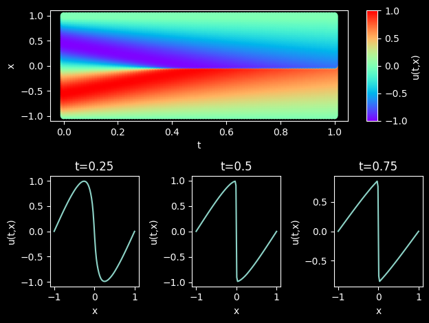
Model Evaluation and Visualization

After training, all data points in the flow field can be inferred. And related results can be visualized.

# visualization
steps = config["train_steps"]
visual_result(model, step=steps, resolution=config["visual_resolution"])