Document feedback

Question document fragment

When a question document fragment contains a formula, it is displayed as a space.

Submission type

issue

It's a little complicated...

I'd like to ask someone.

Please select the submission type

Problem type

Specifications and Common Mistakes

- Specifications and Common Mistakes:

- Misspellings or punctuation mistakes,incorrect formulas, abnormal display.

- Incorrect links, empty cells, or wrong formats.

- Chinese characters in English context.

- Minor inconsistencies between the UI and descriptions.

- Low writing fluency that does not affect understanding.

- Incorrect version numbers, including software package names and version numbers on the UI.

Usability

- Usability:

- Incorrect or missing key steps.

- Missing main function descriptions, keyword explanation, necessary prerequisites, or precautions.

- Ambiguous descriptions, unclear reference, or contradictory context.

- Unclear logic, such as missing classifications, items, and steps.

Correctness

- Correctness:

- Technical principles, function descriptions, supported platforms, parameter types, or exceptions inconsistent with that of software implementation.

- Incorrect schematic or architecture diagrams.

- Incorrect commands or command parameters.

- Incorrect code.

- Commands inconsistent with the functions.

- Wrong screenshots.

- Sample code running error, or running results inconsistent with the expectation.

Risk Warnings

- Risk Warnings:

- Lack of risk warnings for operations that may damage the system or important data.

Content Compliance

- Content Compliance:

- Contents that may violate applicable laws and regulations or geo-cultural context-sensitive words and expressions.

- Copyright infringement.

Please select the type of question

Problem description

Describe the bug so that we can quickly locate the problem.

Submit

Document feedback

FNO for 1D Burgers

  

Overview

Computational fluid dynamics is one of the most important techniques in the field of fluid mechanics in the 21st century. The flow analysis, prediction and control can be realized by solving the governing equations of fluid mechanics by numerical method. Traditional finite element method (FEM) and finite difference method (FDM) are inefficient because of the complex simulation process (physical modeling, meshing, numerical discretization, iterative solution, etc.) and high computing costs. Therefore, it is necessary to improve the efficiency of fluid simulation with AI.

Machine learning methods provide a new paradigm for scientific computing by providing a fast solver similar to traditional methods. Classical neural networks learn mappings between finite dimensional spaces and can only learn solutions related to a specific discretization. Different from traditional neural networks, Fourier Neural Operator (FNO) is a new deep learning architecture that can learn mappings between infinite-dimensional function spaces. It directly learns mappings from arbitrary function parameters to solutions to solve a class of partial differential equations. Therefore, it has a stronger generalization capability. More information can be found in the paper, Fourier Neural Operator for Parametric Partial Differential Equations.

This tutorial describes how to solve the 1-d Burgers’ equation using Fourier neural operator.

Burgers’ equation

The 1-d Burgers’ equation is a non-linear PDE with various applications including modeling the one dimensional flow of a viscous fluid. It takes the form

$${\partial }_{t}u(x,t)+{\partial }_x(u^2(x,t)/2)=\nu {\partial }_{xx}u(x,t),x\in (0,1),t\in (0,1]$$

$$u(x,0)=u_0(x),x\in (0,1)$$

where $u$ is the velocity field, $u_0$ is the initial condition and $\nu$ is the viscosity coefficient.

Problem Description

We aim to learn the operator mapping the initial condition to the solution at time one:

$$u_0\mapsto u(\cdot ,1)$$

Technology Path

MindFlow solves the problem as follows:

1. Training Dataset Construction.

2. Model Construction.

3. Optimizer and Loss Function.

4. Define Solver.

5. Define Callback.

6. Model Training.

Fourier Neural Operator

The Fourier Neural Operator consists of the Lifting Layer, Fourier Layers, and the Decoding Layer.

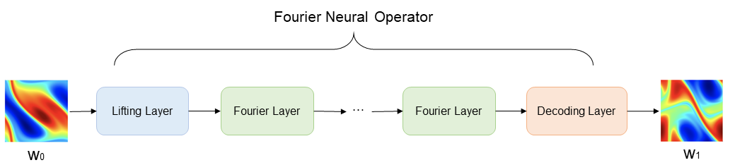
Fourier layers: Start from input V. On top: apply the Fourier transform $\mathcal{F}$; a linear transform R on the lower Fourier modes and filters out the higher modes; then apply the inverse Fourier transform ${\mathcal{F}}^{-1}$. On the bottom: apply a local linear transform W. Finally, the Fourier Layer output vector is obtained through the activation function.

import os

import numpy as np

from mindspore import context, nn, Tensor, set_seed
from mindspore import DynamicLossScaleManager, LossMonitor, TimeMonitor

The following src pacakage can be downloaded in applications/data_driven/burgers/src.

from mindflow import FNO1D, RelativeRMSELoss, Solver, load_yaml_config, get_warmup_cosine_annealing_lr

from src import PredictCallback, create_training_dataset


set_seed(0)
np.random.seed(0)

context.set_context(mode=context.GRAPH_MODE, device_target='GPU', device_id=4)

config = load_yaml_config("burgers1d.yaml")
data_params = config["data"]
model_params = config["model"]
optimizer_params = config["optimizer"]
callback_params = config["callback"]

Training Dataset Construction

Download the training and test dataset: data_driven/burgers/dataset .

In this case, training datasets and test datasets are generated according to Zongyi Li’s dataset in Fourier Neural Operator for Parametric Partial Differential Equations . The settings are as follows:

the initial condition $u_0(x)$ is generated according to periodic boundary conditions:

$$u_0\sim \mu ,\mu =\mathcal{N}(0,625(-\mathrm{\Delta }+25I{)}^{-2})$$

We set the viscosity to $\nu =0.1$ and solve the equation using a split step method where the heat equation part is solved exactly in Fourier space then the non-linear part is advanced, again in Fourier space, using a very fine forward Euler method. The number of samples in the training set is 1000, and the number of samples in the test set is 200.

# create training dataset
train_dataset = create_training_dataset(data_params, shuffle=True)

# create test dataset
test_input, test_label = np.load(os.path.join(data_params["path"], "test/inputs.npy")), \
                         np.load(os.path.join(data_params["path"], "test/label.npy"))

Data preparation finished
input_path:  (1000, 1024, 1)
label_path:  (1000, 1024)

Model Construction

The network is composed of 1 lifting layer, multiple Fourier layers and 1 decoding layer:

• The Lifting layer corresponds to the FNO1D.fc0 in the case, and maps the output data $x$ to the high dimension;

• Multi-layer Fourier Layer corresponds to the FNO1D.fno_seq in the case. Discrete Fourier transform is used to realize the conversion between time domain and frequency domain;

• The Decoding layer corresponds to FNO1D.fc1 and FNO1D.fc2 in the case to obtain the final predictive value.

The initialization of the model based on the network above, parameters can be modified in configuration file.

model = FNO1D(in_channels=model_params["in_channels"],
              out_channels=model_params["out_channels"],
              resolution=model_params["resolution"],
              modes=model_params["modes"],
              channels=model_params["width"],
              depth=model_params["depth"])

Optimizer and Loss Function

steps_per_epoch = train_dataset.get_dataset_size()
lr = get_warmup_cosine_annealing_lr(lr_init=optimizer_params["initial_lr"],
                                    last_epoch=optimizer_params["train_epochs"],
                                    steps_per_epoch=steps_per_epoch,
                                    warmup_epochs=1)
optimizer = nn.Adam(model.trainable_params(), learning_rate=Tensor(lr))
loss_scale = DynamicLossScaleManager()

loss_fn = RelativeRMSELoss()

Define Solver

Solver class is the interface for model training and evaluation. Given the optimizer, network model, loss function, loss scaling strategy, etc. the solver object can be defined easily. Parameters of optimizer_params and model_params can be modified in configuration file.

solver = Solver(model,
                optimizer=optimizer,
                loss_scale_manager=loss_scale,
                loss_fn=loss_fn,
                )

Define Callback

summary_dir = os.path.join(callback_params["summary_dir"], "FNO1D")
print(summary_dir)
pred_cb = PredictCallback(model=model,
                          inputs=test_input,
                          label=test_label,
                          config=config,
                          summary_dir=summary_dir)

./FNO1D
check test dataset shape: (200, 1024, 1), (200, 1024)

Model Training

Invoke the Solver interface for model training and callback interface for evaluation.

solver.train(epoch=optimizer_params["train_epochs"],
             train_dataset=train_dataset,
             callbacks=[LossMonitor(), TimeMonitor(), pred_cb],
             dataset_sink_mode=True)

epoch: 1 step: 125, loss is 2.377823
Train epoch time: 5782.938 ms, per step time: 46.264 ms
epoch: 2 step: 125, loss is 0.88470775
Train epoch time: 1150.446 ms, per step time: 9.204 ms
epoch: 3 step: 125, loss is 0.98071647
Train epoch time: 1135.464 ms, per step time: 9.084 ms
epoch: 4 step: 125, loss is 0.5404751
Train epoch time: 1114.245 ms, per step time: 8.914 ms
epoch: 5 step: 125, loss is 0.39976493
Train epoch time: 1125.107 ms, per step time: 9.001 ms
epoch: 6 step: 125, loss is 0.508416
Train epoch time: 1127.477 ms, per step time: 9.020 ms
epoch: 7 step: 125, loss is 0.42839915
Train epoch time: 1125.775 ms, per step time: 9.006 ms
epoch: 8 step: 125, loss is 0.28270185
Train epoch time: 1118.428 ms, per step time: 8.947 ms
epoch: 9 step: 125, loss is 0.24137405
Train epoch time: 1121.705 ms, per step time: 8.974 ms
epoch: 10 step: 125, loss is 0.22623646
Train epoch time: 1118.699 ms, per step time: 8.950 ms
================================Start Evaluation================================
mean rms_error: 0.03270653011277318
=================================End Evaluation=================================
...
predict total time: 0.5012176036834717 s
epoch: 91 step: 125, loss is 0.026378194
Train epoch time: 1119.095 ms, per step time: 8.953 ms
epoch: 92 step: 125, loss is 0.057838168
Train epoch time: 1116.712 ms, per step time: 8.934 ms
epoch: 93 step: 125, loss is 0.034773324
Train epoch time: 1107.931 ms, per step time: 8.863 ms
epoch: 94 step: 125, loss is 0.029720988
Train epoch time: 1109.336 ms, per step time: 8.875 ms
epoch: 95 step: 125, loss is 0.02933883
Train epoch time: 1111.804 ms, per step time: 8.894 ms
epoch: 96 step: 125, loss is 0.03140598
Train epoch time: 1116.788 ms, per step time: 8.934 ms
epoch: 97 step: 125, loss is 0.03695058
Train epoch time: 1115.020 ms, per step time: 8.920 ms
epoch: 98 step: 125, loss is 0.039841708
Train epoch time: 1120.316 ms, per step time: 8.963 ms
epoch: 99 step: 125, loss is 0.039001673
Train epoch time: 1134.618 ms, per step time: 9.077 ms
epoch: 100 step: 125, loss is 0.038434036
Train epoch time: 1116.549 ms, per step time: 8.932 ms
================================Start Evaluation================================
mean rms_error: 0.005707952339434996
=================================End Evaluation=================================
predict total time: 0.5055065155029297 s