1D Sod Tube

  

This notebook requires MindSpore version >= 2.0.0 to support new APIs including: mindspore.jit, mindspore.jit_class.

The shock tube problem is a common test for the accuracy of computational fluid codes. The test consists of a one-dimensional Riemann problem, i.e, the development of an ideal gas under different conditions at the left and right ends.

Problem Description

The definition of the Sod tube problem is:

$$\begin{array}{r}\frac{\partial }{\partial t}\left(\begin{array}{c}\rho \\ \rho u\\ E\end{array}\right)+\frac{\partial }{\partial x}\left(\begin{array}{c}\rho u\\ \rho u^2+p\\ u(E+p)\end{array}\right)=0\end{array}$$

$$E=\frac{p}{\gamma -1}+\frac{1}{2}\rho u^2$$

where $\gamma =1.4$ for ideal gas. The initial condition is

$$\begin{array}{r}{\left(\begin{array}{c}\rho \\ u\\ p\end{array}\right)}_{x<0.5}=\left(\begin{array}{c}1.0\\ 0.0\\ 1.0\end{array}\right),{\left(\begin{array}{c}\rho \\ u\\ p\end{array}\right)}_{x>0.5}=\left(\begin{array}{c}0.125\\ 0.0\\ 0.1\end{array}\right)\end{array}$$

The Neumann boundary condition is applied on both side of the tube.

The following src pacakage can be downloaded in src.

import mindspore as ms
from mindflow import load_yaml_config, vis_1d
from mindflow import cfd
from mindflow.cfd.runtime import RunTime
from mindflow.cfd.simulator import Simulator

from src.ic import sod_ic_1d

ms.set_context(device_target="GPU", device_id=3)

Defining Simulator and RunTime

The mesh, material, runtime, boundary conditions and numerical methods are defined in numeric.yaml.

config = load_yaml_config('numeric.yaml')
simulator = Simulator(config)
runtime = RunTime(config['runtime'], simulator.mesh_info, simulator.material)

Initial Condition

Initial condition is determined according to mesh coordinates.

mesh_x, _, _ = simulator.mesh_info.mesh_xyz()
pri_var = sod_ic_1d(mesh_x)
con_var = cfd.cal_con_var(pri_var, simulator.material)

Running Simulation

Run CFD simulation with time marching.

while runtime.time_loop(pri_var):
    pri_var = cfd.cal_pri_var(con_var, simulator.material)
    runtime.compute_timestep(pri_var)
    con_var = simulator.integration_step(con_var, runtime.timestep)
    runtime.advance()

current time = 0.000000, time step = 0.007606
current time = 0.007606, time step = 0.005488
current time = 0.013094, time step = 0.004744
current time = 0.017838, time step = 0.004501
current time = 0.022339, time step = 0.004338
current time = 0.026678, time step = 0.004293
current time = 0.030971, time step = 0.004268
current time = 0.035239, time step = 0.004198
current time = 0.039436, time step = 0.004157
current time = 0.043593, time step = 0.004150
current time = 0.047742, time step = 0.004075
current time = 0.051818, time step = 0.004087
current time = 0.055905, time step = 0.004056
current time = 0.059962, time step = 0.004031
current time = 0.063993, time step = 0.004021
current time = 0.068014, time step = 0.004048
current time = 0.072062, time step = 0.004039
current time = 0.076101, time step = 0.004016
current time = 0.080117, time step = 0.004049
current time = 0.084166, time step = 0.004053
current time = 0.088218, time step = 0.004045
current time = 0.092264, time step = 0.004053
current time = 0.096317, time step = 0.004062
current time = 0.100378, time step = 0.004065
current time = 0.104443, time step = 0.004068
current time = 0.108511, time step = 0.004072
current time = 0.112583, time step = 0.004075
current time = 0.116658, time step = 0.004077
current time = 0.120735, time step = 0.004080
current time = 0.124815, time step = 0.004081
...
current time = 0.186054, time step = 0.004084
current time = 0.190138, time step = 0.004084
current time = 0.194222, time step = 0.004084
current time = 0.198306, time step = 0.004085

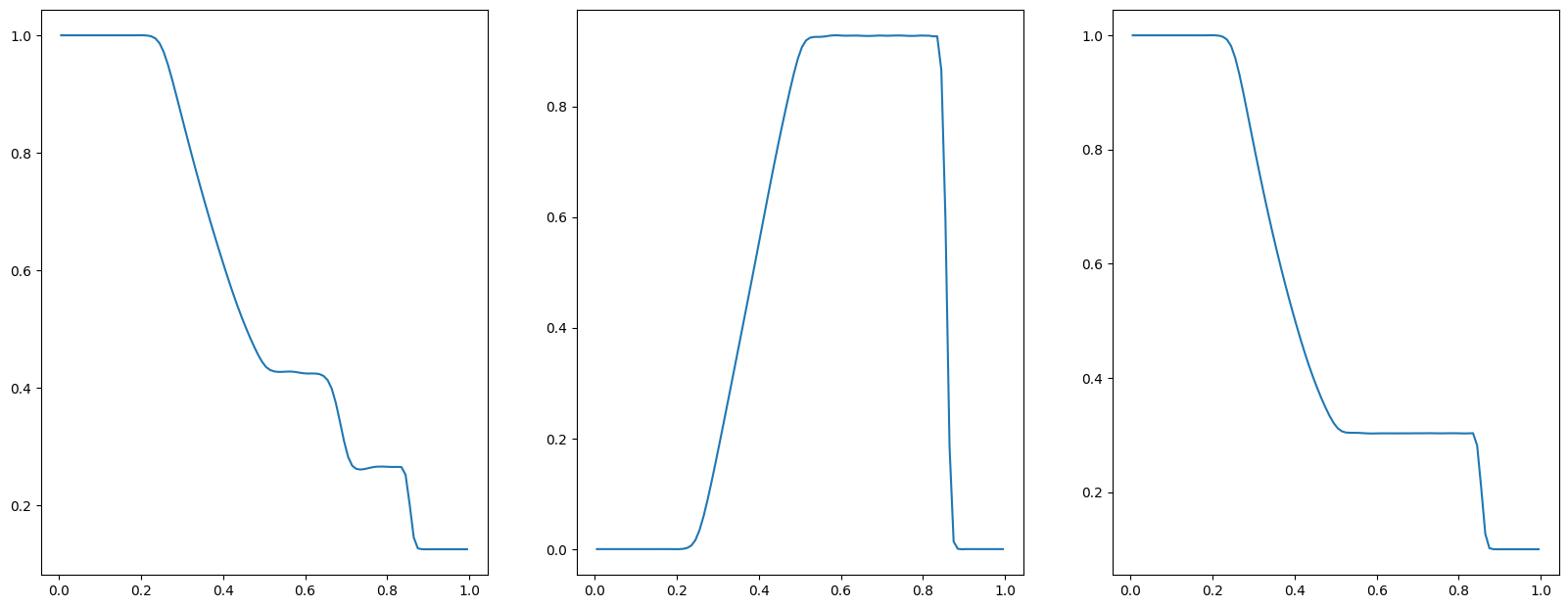
Post Processing

You can view the density, pressure and velocity.

pri_var = cfd.cal_pri_var(con_var, simulator.material)
vis_1d(pri_var, 'sod.jpg')