Multi-copy Parallel

Overview

In large model training, communication introduced by tensor parallel is a significant performance bottleneck. This part of communication depends on the previous calculation result and cannot be overlapped with the calculation. To solve this problem, mindspore proposes multi-copy parallel.

Usage Scenario: When there is model parallel in semi-automatic mode as well as in the network, the forward computation of the 1st copy of the sliced data will be performed at the same time as the 2nd copy of the data will be communicated with the parallel model as a way to achieve performance acceleration of the communication and computation concurrency.

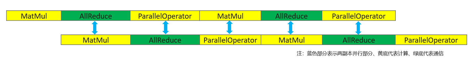
Basic Principle

The data of input model is sliced according to the batchsize dimension, thus modifying the existing single-copy form into a multi-copy form, so that when the underlying layer is communicating, the other copy carries out the computational operation without waiting, which ensures that the computation and communication times of multi-copy complement each other and improve the model performance. At the same time, splitting the data into a multi-copy form also reduces the number of parameter of the operator inputs and reduces the computation time of a single operator, which is helpful in improving the model performance.

Related Interfaces

• mindspore.nn.MicroBatchInterleaved(cell_network, interleave_num=2): This function serves to split the input into interleave_num parts in the zeroth dimension, and then performs the computation of the wrapped cell.

Operator Practice

The following is an illustration of multi-copy parallel operation using an Ascend or GPU stand-alone 8-card example:

Example Code Description

Download the complete example code:multiple_copy.

The directory structure is as follows:

└─ sample_code
    ├─ multiple_copy
       ├── train.py
       └── run.sh
    ...

train.py is the script that defines the network structure and the training process. run.sh is the execution script.

Configuring a Distributed Environment

Initialize HCCL communication with init.

import mindspore as ms
from mindspore.communication import init

ms.set_context(mode=ms.GRAPH_MODE)
init()

Dataset Loading and Network Definition

Here the dataset loading and network definition is consistent with the single-card model. Defer initialization of network parameters and optimizer parameters via the no_init_parameters interface.

import os
import mindspore.dataset as ds
from mindspore import nn
from mindspore.nn.utils import no_init_parameters

def create_dataset(batch_size):
    dataset_path = os.getenv("DATA_PATH")
    dataset = ds.MnistDataset(dataset_path)
    image_transforms = [
        ds.vision.Rescale(1.0 / 255.0, 0),
        ds.vision.Normalize(mean=(0.1307,), std=(0.3081,)),
        ds.vision.HWC2CHW()
    ]
    label_transform = ds.transforms.TypeCast(ms.int32)
    dataset = dataset.map(image_transforms, 'image')
    dataset = dataset.map(label_transform, 'label')
    dataset = dataset.batch(batch_size)
    return dataset

data_set = create_dataset(32)

class Network(nn.Cell):
    def __init__(self):
        super().__init__()
        self.flatten = nn.Flatten()
        self.dense_relu_sequential = nn.SequentialCell(
            nn.Dense(28*28, 512, weight_init="normal", bias_init="zeros"),
            nn.ReLU(),
            nn.Dense(512, 512, weight_init="normal", bias_init="zeros"),
            nn.ReLU(),
            nn.Dense(512, 10, weight_init="normal", bias_init="zeros")
        )

    def construct(self, x):
        x = self.flatten(x)
        logits = self.dense_relu_sequential(x)
        return logits

with no_init_parameters():
    net = Network()
    optimizer = nn.SGD(net.trainable_params(), 1e-2)

Training the Network

In this step, we need to define the loss function and the training process, and in this section two interfaces need to be called to configure the gradient accumulation:

• First the LossCell needs to be defined. In this case the nn.WithLossCell interface is called to wrap the network and loss functions.

• It is then necessary to wrap a layer of mindspore.parallel.MicroBatchInterleaved around the LossCell and specify interleave_num size of 2. Refer to the relevant interfaces in the overview of this chapter for more details.

Finally, the AutoParallel wraps net and sets the parallel mode to semi-automatic parallel mode.

import mindspore as ms
from mindspore import nn, train

loss_fn = nn.CrossEntropyLoss()
loss_cb = train.LossMonitor(100)
net = ms.parallel.MicroBatchInterleaved(nn.WithLossCell(net, loss_fn), 2)
net = AutoParallel(net, parallel_mode="semi_auto")
model = ms.Model(net, optimizer=optimizer)
model.train(10, data_set, callbacks=[loss_cb])

Multi-copy parallel training is more suitable to use model.train approach, this is because the TrainOneStep logic under multi-copy parallel is complex, while model.train internally encapsulates the TrainOneStepCell for multi-copy parallel, which is much easier to use.

Running Stand-alone 8-card Script

Next, the corresponding script is called by the command. Take the msrun startup method, the 8-card distributed training script as an example, and perform the distributed training:

bash run.sh

After training, the part of results about the Loss are saved in log_output/worker_*.log. The example is as follows:

epoch: 1 step: 100, loss is 4.514171123504639
epoch: 1 step: 200, loss is 3.835113048553467
epoch: 1 step: 300, loss is 1.9824411869049072
epoch: 1 step: 400, loss is 1.2429465055465698
epoch: 1 step: 500, loss is 1.0608973503112793
epoch: 1 step: 600, loss is 0.9407652616500854
epoch: 1 step: 700, loss is 0.8292769193649292
...