Differences Between MindSpore and PyTorch

Differences Between MindSpore and PyTorch APIs

torch.device

When building a model, PyTorch usually uses torch.device to specify the device to which the model and data are bound, that is, whether the device is on the CPU or GPU. If multiple GPUs are supported, you can also specify the GPU sequence number. After binding a device, you need to deploy the model and data to the device. The code is as follows:

import os
import torch
from torch import nn

# bind to the GPU 0 if GPU is available, otherwise bind to CPU
device = torch.device("cuda:0" if torch.cuda.is_available() else "cpu") # Single GPU or CPU
# deploy model to specified hardware
model.to(device)
# deploy data to specified hardware
data.to(device)

# distribute training on multiple GPUs
if torch.cuda.device_count() > 1:
    model = nn.DataParallel(model, device_ids=[0,1,2])
    model.to(device)

    # set available device
    os.environ['CUDA_VISIBLE_DEVICE']='1'
    model.cuda()

In MindSpore, the device_target parameter in context specifies the device bound to the model, and the device_id parameter specifies the device sequence number. Different from PyTorch, once the device is successfully set, the input data and model are copied to the specified device for execution by default. You do not need to and cannot change the type of the device where the data and model run. The sample code is as follows:

import mindspore as ms
ms.set_context(device_target='Ascend', device_id=0)

# define net
Model = ..
# define dataset
dataset = ..
# training, automatically deploy to Ascend according to device_target
Model.train(1, dataset)

In addition, the Tensor returned after the network runs is copied to the CPU device by default. You can directly access and modify the Tensor, including converting the Tensor to the numpy format. Unlike PyTorch, you do not need to run the tensor.cpu command and then convert the Tensor to the NumPy format.

nn.Module

When PyTorch is used to build a network structure, the nn.Module class is used. Generally, network elements are defined and initialized in the __init__ function, and the graph structure expression of the network is defined in the forward function. Objects of these classes are invoked to build and train the entire model. nn.Module not only provides us with graph building interfaces, but also provides us with some common APIs to help us execute more complex logic.

The nn.Cell class in MindSpore plays the same role as the nn.Module class in PyTorch. Both classes are used to build graph structures. MindSpore also provides various APIs for developers. Although the names are not the same, the mapping of common functions in nn.Module can be found in nn.Cell.

The following uses several common methods as examples:

Common Method	nn.Module	nn.Cell
Obtain child elements.	named_children	cells_and_names
Add subelements.	add_module	insert_child_to_cell
Obtain parameters of an element.	parameters	get_parameters

Data Size

In PyTorch, there are four types of objects that can store data: Tensor, Variable, Parameter, and Buffer. The default behaviors of the four types of objects are different. When the gradient is not required, the Tensor and Buffer data objects are used. When the gradient is required, the Variable and Parameter data objects are used. When PyTorch designs the four types of data objects, the functions are redundant. (In addition, Variable will be discarded.)

MindSpore optimizes the data object design logic and retains only two types of data objects: Tensor and Parameter. The Tensor object only participates in calculation and does not need to perform gradient derivation or parameter update on it. The Parameter data object has the same meaning as the Parameter data object of PyTorch. The requires_grad attribute determines whether to perform gradient derivation or parameter update on the Parameter data object. During network migration, all data objects that are not updated in PyTorch can be declared as Tensor in MindSpore.

Gradient Derivation

The operator and interface differences involved in gradient derivation are mainly caused by different automatic differentiation principles of MindSpore and PyTorch.

torch.no_grad

In PyTorch, by default, information required for backward propagation is recorded when forward computation is performed. In the inference phase or in a network where backward propagation is not required, this operation is redundant and time-consuming. Therefore, PyTorch provides torch.no_grad to cancel this process.

MindSpore constructs a backward graph based on the forward graph structure only when GradOperation is invoked. No information is recorded during forward execution. Therefore, MindSpore does not need this interface. It can be understood that forward calculation of MindSpore is performed in torch.no_grad mode.

retain_graph

PyTorch is function-based automatic differentiation. Therefore, by default, the recorded information is automatically cleared after each backward propagation is performed for the next iteration. As a result, when we want to reuse the backward graph and gradient information, the information fails to be obtained because it has been deleted. Therefore, PyTorch provides backward(retain_graph=True) to proactively retain the information.

MindSpore does not require this function. MindSpore is an automatic differentiation based on the computational graph. The backward graph information is permanently recorded in the computational graph after GradOperation is invoked. You only need to invoke the computational graph again to obtain the gradient information.

High-order Derivatives

Automatic differentiation based on computational graphs also has an advantage that we can easily implement high-order derivation. After the GradOperation operation is performed on the forward graph for the first time, a first-order derivative may be obtained. In this case, the computational graph is updated to a backward graph structure of the forward graph + the first-order derivative. However, after the GradOperation operation is performed on the updated computational graph again, a second-order derivative may be obtained, and so on. Through automatic differentiation based on computational graph, we can easily obtain the higher order derivative of a network.

Differences Between MindSpore and PyTorch Operators

Most operators and APIs of MindSpore are similar to those of TensorFlow, but the default behavior of some operators is different from that of PyTorch or TensorFlow. During network script migration, if developers do not notice these differences and directly use the default behavior, the network may be inconsistent with the original migration network, affecting network training. It is recommended that developers align not only the used operators but also the operator attributes during network migration. Here we summarize several common difference operators.

nn.Dropout

Dropout is often used to prevent training overfitting. It has an important probability value parameter. The meaning of this parameter in MindSpore is completely opposite to that in PyTorch and TensorFlow.

In MindSpore, the probability value corresponds to the keep_prob attribute of the Dropout operator, indicating the probability that the input is retained. 1-keep_prob indicates the probability that the input is set to 0.

In PyTorch and TensorFlow, the probability values correspond to the attributes p and rate of the Dropout operator, respectively. They indicate the probability that the input is set to 0, which is opposite to the meaning of keep_prob in MindSpore.nn.Dropout.

For more information, visit MindSpore Dropout, PyTorch Dropout, and TensorFlow Dropout.

nn.BatchNorm2d

BatchNorm is a special regularization method in the CV field. It has different computation processes during training and inference and is usually controlled by operator attributes. BatchNorm of MindSpore and PyTorch uses two different parameter groups at this point.

• Difference 1

torch.nn.BatchNorm2d status under different parameters

training	track_running_stats	Status
True	True	Expected training status. running_mean and running_var trace the statistical features of the batch in the entire training process. Each group of input data is normalized based on the mean and var statistical features of the current batch, and then running_mean and running_var are updated.
True	False	Each group of input data is normalized based on the statistics feature of the current batch, but the running_mean and running_var parameters do not exist.
False	True	Expected inference status. The BN uses running_mean and running_var for normalization and does not update them.
False	False	The effect is the same as that of the second status. The only difference is that this is the inference status and does not learn the weight and bias parameters. Generally, this status is not used.

mindspore.nn.BatchNorm2d status under different parameters

use_batch_statistics	Status
True	Expected training status. moving_mean and moving_var trace the statistical features of the batch in the entire training process. Each group of input data is normalized based on the mean and var statistical features of the current batch, and then moving_mean and moving_var are updated.
Fasle	Expected inference status. The BN uses moving_mean and moving_var for normalization and does not update them.
None	use_batch_statistics is automatically set. For training, set use_batch_statistics to True. For inference, set use_batch_statistics to False.

Compared with torch.nn.BatchNorm2d, mindspore.nn.BatchNorm2d does not have two redundant states and retains only the most commonly used training and inference states.

• Difference 2

The meaning of the momentum parameter of the BatchNorm series operators in MindSpore is opposite to that in PyTorch. The relationship is as follows:

\[momentum_{pytorch} = 1 - momentum_{mindspore}\]

References: mindspore.nn.BatchNorm2d, torch.nn.BatchNorm2d

ops.Transpose

During axis transformation, PyTorch usually uses two operators: Tensor.permute and torch.transpose. MindSpore and TensorFlow provide only the transpose operator. Note that the Tensor.permute contains the functions of the torch.transpose. The torch.transpose supports only the exchange of two axes at the same time, whereas the Tensor.permute supports the exchange of multiple axes at the same time.

# PyTorch code
import numpy as np
import torch
from torch import Tensor
data = np.empty((1, 2, 3, 4)).astype(np.float32)
ret1 = torch.transpose(Tensor(data), dim0=0, dim1=3)
print(ret1.shape)
ret2 = Tensor(data).permute((3, 2, 1, 0))
print(ret2.shape)

    torch.Size([4, 2, 3, 1])
    torch.Size([4, 3, 2, 1])

The transpose operator of MindSpore has the same function as that of TensorFlow. Although the operator is named transpose, it can transform multiple axes at the same time, which is equivalent to Tensor.permute. Therefore, MindSpore does not provide operators similar to torch.tranpose.

# MindSpore code
import mindspore as ms
import numpy as np
from mindspore import ops
ms.set_context(device_target="CPU")
data = np.empty((1, 2, 3, 4)).astype(np.float32)
ret = ops.Transpose()(ms.Tensor(data), (3, 2, 1, 0))
print(ret.shape)

    (4, 3, 2, 1)

For more information, visit MindSpore Transpose, PyTorch Transpose, PyTorch Permute, and TensforFlow Transpose.

Conv and Pooling

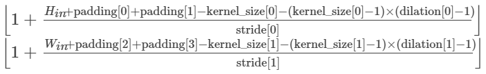
For operators similar to convolution and pooling, the size of the output feature map of the operator depends on variables such as the input feature map, step, kernel_size, and padding.

If pad_mode is set to valid, the height and width of the output feature map are calculated as follows:

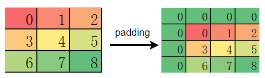
If pad_mode (corresponding to the padding attribute in PyTorch, which has a different meaning from pad_mode) is set to same, automatic padding needs to be performed on the input feature map sometimes. When the padding element is an even number, padding elements are evenly distributed on the top, bottom, left, and right of the feature map. In this case, the behavior of this type of operators in MindSpore, PyTorch, and TensorFlow is the same.

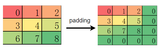
However, when the padding element is an odd number, PyTorch is preferentially filled on the left and upper sides of the input feature map.

MindSpore and TensorFlow are preferentially filled on the right and bottom of the feature map.

The following is an example:

# mindspore example
import numpy as np
import mindspore as ms
from mindspore import ops
ms.set_context(device_target="CPU")
data = np.arange(9).reshape(1, 1, 3, 3).astype(np.float32)
print(data)
op = ops.MaxPool(kernel_size=2, strides=2, pad_mode='same')
print(op(ms.Tensor(data)))

    [[[[0. 1. 2.]
       [3. 4. 5.]
       [6. 7. 8.]]]]
    [[[[4. 5.]
       [7. 8.]]]]

During MindSpore model migration, if the PyTorch pre-training model is loaded to the model and fine-tune is performed in MindSpore, the difference may cause precision decrease. Developers need to pay special attention to the convolution whose padding policy is same.

To keep consistent with the PyTorch behavior, you can use the ops.Pad operator to manually pad elements, and then use the convolution and pooling operations when pad_mode="valid" is set.

import numpy as np
import mindspore as ms
from mindspore import ops
ms.set_context(device_target="CPU")
data = np.arange(9).reshape(1, 1, 3, 3).astype(np.float32)
# only padding on top left of feature map
pad = ops.Pad(((0, 0), (0, 0), (1, 0), (1, 0)))
data = pad(ms.Tensor(data))
res = ops.MaxPool(kernel_size=2, strides=2, pad_mode='vaild')(data)
print(res)

    [[[[0. 2.]
       [6. 8.]]]]

Different Default Weight Initialization

We know that weight initialization is very important for network training. Generally, each operator has an implicit declaration weight. In different frameworks, the implicit declaration weight may be different. Even if the operator functions are the same, if the implicitly declared weight initialization mode distribution is different, the training process is affected or even cannot be converged.

Common operators that implicitly declare weights include Conv, Dense(Linear), Embedding, and LSTM. The Conv and Dense operators differ greatly.

• Conv2d

  • mindspore.nn.Conv2d (weight: \(\mathcal{N} (0, 1) \), bias: zeros)

  • torch.nn.Conv2d (weight: \(\mathcal{U} (-\sqrt{k},\sqrt{k} )\), bias: \(\mathcal{U} (-\sqrt{k},\sqrt{k} )\))

  • tf.keras.Layers.Conv2D (weight: glorot_uniform, bias: zeros)

  In the preceding information, \(k=\frac{groups}{c_{in}*\prod_{i}^{}{kernel\_size[i]}}\)

• Dense(Linear)

  • mindspore.nn.Linear (weight: \(\mathcal{N} (0, 1) \), bias: zeros)

  • torch.nn.Dense (weight: \(\mathcal{U} (-\sqrt{k},\sqrt{k} )\), bias: \(\mathcal{U} (-\sqrt{k},\sqrt{k} )\))

  • tf.keras.Layers.Dense (weight: glorot_uniform, bias: zeros)

  In the preceding information, \(k=\frac{groups}{in\_features}\)

For a network without normalization, for example, a GAN network without the BatchNorm operator, the gradient is easy to explode or disappear. Therefore, weight initialization is very important. Developers should pay attention to the impact of weight initialization.

Differences Between MindSpore and PyTorch Execution Processes

Automatic Differentiation

Both MindSpore and PyTorch provide the automatic differentiation function. After the forward network is defined, automatic backward propagation and gradient update can be implemented through simple interface invoking. However, it should be noted that MindSpore and PyTorch use different logic to build backward graphs. This difference also brings differences in API design.

PyTorch Automatic Differentiation

As we know, PyTorch is an automatic differentiation based on computation path tracing. After a network structure is defined, no backward graph is created. Instead, during the execution of the forward graph, Variable or Parameter records the backward function corresponding to each forward computation and generates a dynamic computational graph, it is used for subsequent gradient calculation. When backward is called at the final output, the chaining rule is applied to calculate the gradient from the root node to the leaf node. The nodes stored in the dynamic computational graph of PyTorch are actually Function objects. Each time an operation is performed on Tensor, a Function object is generated, which records necessary information in backward propagation. During backward propagation, the autograd engine calculates gradients in backward order by using the backward of the Function. You can view this point through the hidden attribute of the Tensor.

For example, run the following code:

import torch
from torch.autograd import Variable
x = Variable(torch.ones(2, 2), requires_grad=True)
x = x * 2
y = x - 1
y.backward(x)

The gradient result of x in the process from obtaining the definition of x to obtaining the output y is automatically obtained.

Note that the backward of PyTorch is accumulated. After the update, you need to clear the optimizer.

MindSpore Automatic Differentiation

In graph mode, MindSpore’s automatic differentiation is based on the graph structure. Different from PyTorch, MindSpore does not record any information during forward computation and only executes the normal computation process (similar to PyTorch in PyNative mode). Then the question comes. If the entire forward computation is complete and MindSpore does not record any information, how does MindSpore know how backward propagation is performed?

When MindSpore performs automatic differentiation, the forward graph structure needs to be transferred. The automatic differentiation process is to obtain backward propagation information by analyzing the forward graph. The automatic differentiation result is irrelevant to the specific value in the forward computation and is related only to the forward graph structure. Through the automatic differentiation of the forward graph, the backward propagation process is obtained. The backward propagation process is expressed through a graph structure, that is, the backward graph. The backward graph is added after the user-defined forward graph to form a final computational graph. However, the backward graph and backward operators added later are not aware of and cannot be manually added. They can only be automatically added through the interface provided by MindSpore. In this way, errors are avoided during backward graph build.

Finally, not only the forward graph is executed, but also the graph structure contains both the forward operator and the backward operator added by MindSpore. That is, MindSpore adds an invisible Cell after the defined forward graph, the Cell is a backward operator derived from the forward graph.

The interface that helps us build the backward graph is GradOperation.

from mindspore import nn, ops

class GradNetWrtX(nn.Cell):
    def __init__(self, net):
        super(GradNetWrtX, self).__init__()
        self.net = net
        self.grad_op = ops.GradOperation()
    def construct(self, x, y):
        gradient_function = self.grad_op(self.net)
        return gradient_function(x, y)

According to the document introduction, GradOperation is not an operator. Its input and output are not tensors, but cells, that is, the defined forward graph and the backward graph obtained through automatic differentiation. Why is the input a graph structure? To construct a backward graph, you do not need to know the specific input data. You only need to know the structure of the forward graph. With the forward graph, you can calculate the structure of the backward graph. Then, you can treat the forward graph and backward graph as a new computational graph, the new computational graph is like a function. For any group of data you enter, it can calculate not only the positive output, but also the gradient of ownership weight. Because the graph structure is fixed and does not save intermediate variables, the graph structure can be invoked repeatedly.

Similarly, when we add an optimizer structure to the network, the optimizer also adds optimizer-related operators. That is, we add optimizer operators that are not perceived to the computational graph. Finally, the computational graph is built.

In MindSpore, most operations are finally converted into real operator operations and finally added to the computational graph. Therefore, the number of operators actually executed in the computational graph is far greater than the number of operators defined at the beginning.

MindSpore provides the TrainOneStepCell and TrainOneStepWithLossScaleCell APIs to package the entire training process. If other operations, such as gradient cropping, specification, and intermediate variable return, are performed in addition to the common training process, you need to customize the training cell. For details, see Inference and Training Process.

Learning Rate Update

PyTorch Learning Rate (LR) Update Policy

PyTorch provides the torch.optim.lr_scheduler package for dynamically modifying LR. When using the package, you need to explicitly call optimizer.step() and scheduler.step() to update LR. For details, see How Do I Adjust the Learning Rate.

MindSpore Learning Rate Update Policy

The learning rate of MindSpore is packaged in the optimizer. Each time the optimizer is invoked, the learning rate update step is automatically updated. For details, see Learning Rate and Optimizer.

Distributed Scenarios

PyTorch Distributed Settings

Generally, data parallelism is used in distributed scenarios. For details, see DDP. The following is an example of PyTorch:

import os
import torch
import torch.distributed as dist
import torch.multiprocessing as mp
import torch.nn as nn
import torch.optim as optim
from torch.nn.parallel import DistributedDataParallel as DDP


def example(rank, world_size):
    # create default process group
    dist.init_process_group("gloo", rank=rank, world_size=world_size)
    # create local model
    model = nn.Linear(10, 10).to(rank)
    # construct DDP model
    ddp_model = DDP(model, device_ids=[rank])
    # define loss function and optimizer
    loss_fn = nn.MSELoss()
    optimizer = optim.SGD(ddp_model.parameters(), lr=0.001)

    # forward pass
    outputs = ddp_model(torch.randn(20, 10).to(rank))
    labels = torch.randn(20, 10).to(rank)
    # backward pass
    loss_fn(outputs, labels).backward()
    # update parameters
    optimizer.step()

def main():
    world_size = 2
    mp.spawn(example,
        args=(world_size,),
        nprocs=world_size,
        join=True)

if __name__=="__main__":
    # Environment variables which need to be
    # set when using c10d's default "env"
    # initialization mode.
    os.environ["MASTER_ADDR"] = "localhost"
    os.environ["MASTER_PORT"] = "29500"
    main()

MindSpore Distributed Settings

The distributed configuration of MindSpore uses runtime configuration items. For details, see Distributed Parallel Training Mode. For example:

import mindspore as ms
from mindspore.communication.management import init, get_rank, get_group_size

# Initialize the multi-device environment.
init()

# Obtain the number of devices in a distributed scenario and the logical ID of the current process.
group_size = get_group_size()
rank_id = get_rank()

# Configure data parallel mode in distributed mode.
ms.set_auto_parallel_context(parallel_mode=ms.ParallelMode.DATA_PARALLEL, gradients_mean=True)