Higher-order Operator-level Parallelism

Overview

Operator-level Parallelism is a commonly used parallelism technique in large model training inference, which can slice the tensor across multiple cards and effectively reduce GPU memory on a single card. MindSpore is configured for operator-level parallelism by describing tensor slicing in tuples for each input of the operator through mindspore.ops.Primitive.shard() interface, which is easy to configure for most scenarios. Accordingly, this type of slicing only describes the tensor slicing but shields the tensor layout on the device rank from the users, and thus expresses a limited mapping between tensor slicing and device ranking, which cannot support slicing for some more complex scenarios. Therefore, this tutorial will introduce an operator-level parallel configuration method of the open device layout description.

Hardware platforms supported for advanced operator-level parallel models include Ascend, GPUs, and need to be run in Graph mode.

Background

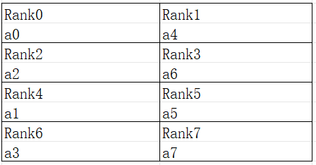
Operator-level Parallelism describes MindSpore basic slicing logic for tensors, but cannot express all the slicing scenarios. For a 2D tensor "[[a0, a1, a2, a3], [a4, a5, a6, a7]]", the tensor layout is shown below:

Figure: Schematic of 2D tensor arrangement

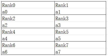
It can be seen that the 0-axis of the tensor, e.g. "[a0, a1, a2, a3]" slices to the discontinuous card "[Rank0, Rank4, Rank2, Rank6]" and the tensor is sliced according to strategy=(2, 4), the arrangement should be as follows:

Figure: Schematic of a 2D tensor arranged according to a sharding strategy

As can be seen from the above example, directly slicing the input and output tensor of the operator according to the number of slices fails to express some slicing scenarios with special statements.

Interface Configuration

In order to express sharding as in the above scenario, functional extensions are made to the shard interface.

The parameters in_strategy and out_strategy both additionally receive the new quantity type tuple(Layout) type. Layout is initialized using the device matrix, while requiring an alias for each axis of the device matrix, such as " layout = Layout((8, 4, 4), name = ("dp", "sp", "mp"))".

The device matrix describes a total of 128 cards arranged in the shape of (8, 4, 4), and each axis is aliased to "dp", "sp", "mp", and the call to the Layout passes in these axes, and each tensor selects the axes of each dimension according to its shape to map to the device, and also determines the number of copies, such as here "dp" denotes 8 cuts within 8 devices in the highest dimension of the device layout, "sp" denotes 4 cuts within 4 devices in the middle dimension of the device layout, and "mp" denotes 4 cuts within 4 devices in the lowest dimension of the device layout. In particular, one dimension of the tensor may be mapped to multiple dimensions of the device to express multiple slices in one dimension.

The above example of "[[a0, a1, a2, a3], [a4, a5, a6, a7]]" sliced to discontinuous cards can be expressed by Layout as follows:

from mindspore import Layout
a = [[a0, a1, a2, a3], [a4, a5, a6, a7]]
layout = Layout((2, 2, 2), name = ("dp", "sp", "mp"))
a_strategy = layout("mp", ("sp", "dp"))

Notice that the "[a0, a1, a2, a3]" of the tensor a is sliced twice to the "sp" and "mp" axes of the device, so that the result comes out as:

The following is exemplified by a concrete example in which the user computes a two-dimensional matrix multiplication over 8 cards: Y = (X * W) , where the devices are organized according to 2 * 2 * 2, and the cut of X coincides with the cut of the tensor a described above:

import mindspore.nn as nn
from mindspore import ops, Layout
import mindspore as ms

ms.set_auto_parallel_context(parallel_mode=ms.ParallelMode.SEMI_AUTO_PARALLEL, device_num=8)

class DenseMatMulNet(nn.Cell):
    def __init__(self):
        super(DenseMatMulNet, self).__init__()
        layout = Layout((2, 2, 2), name = ("dp", "sp", "mp"))
        in_strategy = (layout("mp", ("sp", "dp")), layout(("sp", "dp"), "None"))
        out_strategy = (layout(("mp", "sp", "dp"), "None"), )
        self.matmul1 = ops.MatMul().shard(in_strategy, out_strategy)
    def construct(self, x, w):
        y = self.matmul1(x, w)
        return y

Operation Practice

The following is an illustration of operator-level parallel operation using an Ascend or GPU standalone 8-card example:

Sample Code Description

Download the complete sample code: distributed_operator_parallel.

The directory structure is as follows:

└─ sample_code
    ├─ distributed_operator_parallel
       ├── advanced_distributed_operator_parallel.py
       ├── run_advanced.sh
       └── ...
    ...

advanced_distributed_operator_parallel.py is the script that defines the network structure and training process. run_advanced.sh is the execution script.

Configuring a Distributed Environment

Specify the run mode, run device, and run card number through the context interface. Unlike single-card scripts, parallel scripts also need to specify the parallel mode parallel_mode to be semi-automatic parallel mode and initialize HCCL or NCCL communication through init. max_device_memory limits the maximum amount of device memory of the model, in order to leave enough device memory for communication on the Ascend hardware platform, GPUs do not need to be reserved. If device_target is not set here, it is automatically specified as the backend hardware device corresponding to the MindSpore package.

import mindspore as ms
from mindspore.communication import init

ms.set_context(mode=ms.GRAPH_MODE)
ms.set_context(max_device_memory="28GB")
ms.set_auto_parallel_context(parallel_mode=ms.ParallelMode.SEMI_AUTO_PARALLEL)
init()
ms.set_seed(1)

Loading Dataset

In the operator-level parallel scenario, the dataset is loaded in the same way as a single card is loaded, with the following code:

import os
import mindspore.dataset as ds

def create_dataset(batch_size):
    dataset_path = os.getenv("DATA_PATH")
    dataset = ds.MnistDataset(dataset_path)
    image_transforms = [
        ds.vision.Rescale(1.0 / 255.0, 0),
        ds.vision.Normalize(mean=(0.1307,), std=(0.3081,)),
        ds.vision.HWC2CHW()
    ]
    label_transform = ds.transforms.TypeCast(ms.int32)
    dataset = dataset.map(image_transforms, 'image')
    dataset = dataset.map(label_transform, 'label')
    dataset = dataset.batch(batch_size)
    return dataset

data_set = create_dataset(32)

Defining the Network

In the current semi-automatic parallel mode, it is necessary to define the network with ops operators (Primitive). The user can manually configure some operator sharding strategy based on single card network. For example, the network structure after configuring the strategy is:

import mindspore as ms
from mindspore import nn, ops

class Network(nn.Cell):
    def __init__(self):
        super().__init__()
        self.flatten = ops.Flatten()
        self.fc1_weight = ms.Parameter(initializer("normal", [28*28, 512], ms.float32))
        self.fc2_weight = ms.Parameter(initializer("normal", [512, 512], ms.float32))
        self.fc3_weight = ms.Parameter(initializer("normal", [512, 10], ms.float32))
        self.matmul1 = ops.MatMul()
        self.relu1 = ops.ReLU()
        self.matmul2 = ops.MatMul()
        self.relu2 = ops.ReLU()
        self.matmul3 = ops.MatMul()

    def construct(self, x):
        x = self.flatten(x)
        x = self.matmul1(x, self.fc1_weight)
        x = self.relu1(x)
        x = self.matmul2(x, self.fc2_weight)
        x = self.relu2(x)
        logits = self.matmul3(x, self.fc3_weight)
        return logits

net = Network()
layout = Layout((2, 2, 2), ("dp", "sp", "mp"))
net.matmul1.shard((layout("mp", ("sp", "dp")), layout(("sp", "dp"), "None")))
net.relu1.shard(((4, 1),))
layout2 = Layout((8,), ("tp",))
net.matmul2.shard((layout2("None", "tp"), layout2("tp", "None")))
net.relu2.shard(((8, 1),))

The ops.MatMul() and ops.ReLU() operators of the above networks are configured with a sharding strategy, where net.matmul1 is also consistent with the sharding arrangement of tensor a above, and net.matmul2 is sliced into 8 parts at the Reduce axis of MatMul.

Training the Network

In this step, we need to define the loss function, the optimizer, and the training process, which is partially the same as that of the single card:

import mindspore as ms
from mindspore import nn

optimizer = nn.SGD(net.trainable_params(), 1e-2)
loss_fn = nn.CrossEntropyLoss()

def forward_fn(data, target):
    logits = net(data)
    loss = loss_fn(logits, target)
    return loss, logits

grad_fn = ms.value_and_grad(forward_fn, None, net.trainable_params(), has_aux=True)

@ms.jit
def train_step(inputs, targets):
    (loss_value, _), grads = grad_fn(inputs, targets)
    optimizer(grads)
    return loss_value

for epoch in range(10):
    i = 0
    for image, label in data_set:
        loss_output = train_step(image, label)
        if i % 10 == 0:
            print("epoch: %s, step: %s, loss is %s" % (epoch, i, loss_output))
        i += 1

Running a Standalone 8-Card Script

Next, the corresponding scripts are called by commands, using the mpirun startup method and the 8-card distributed training script as an example of distributed training:

bash run_advanced.sh

After training, the log files are saved to the log_output directory, and the part of the file directory structure is as follows:

└─ log_output
    └─ 1
        ├─ rank.0
        |   └─ stdout
        ├─ rank.1
        |   └─ stdout
...

The results on the Loss section are saved in log_output/1/rank.*/stdout, and the example is as below:

epoch: 0, step: 0, loss is 2.3016002
epoch: 0, step: 10, loss is 2.2889402
epoch: 0, step: 20, loss is 2.2848126
epoch: 0, step: 30, loss is 2.248126
epoch: 0, step: 40, loss is 2.1581488
epoch: 0, step: 50, loss is 1.8051043
epoch: 0, step: 60, loss is 1.571685
epoch: 0, step: 70, loss is 1.267063
epoch: 0, step: 80, loss is 0.9873328
epoch: 0, step: 90, loss is 0.7807965
...

Other startup methods such as dynamic networking and rank table startup can be found in startup methods.