Performance Profiling (Ascend)

Overview

This article describes how to use MindSpore Profiler for performance debugging on Ascend AI processors.

Operation Process

Prepare a training script, add profiler APIs in the training script and run the training script.
Start MindSpore Insight and specify the summary-base-dir using startup parameters, note that summary-base-dir is the parent directory of the directory created by Profiler. For example, the directory created by Profiler is /home/user/code/data/, the summary-base-dir should be /home/user/code. After MindSpore Insight is started, access the visualization page based on the IP address and port number. The default access IP address is http://127.0.0.1:8080.
Find the training in the list, click the performance profiling link and view the data on the web page.

Preparing the Training Script

There are two ways to collect neural network performance data. You can enable Profiler in either of the following ways.

Method 1: Modify the training script

Add the MindSpore Profiler interface to the training script.

Before training, initialize the MindSpore Profiler object, and profiler enables collection of performance data.

Note

The parameters of Profiler are as follows: Profiler API . Before initializing the Profiler, you need to determine the device_id.
At the end of the training, Profiler.analyse() should be called to finish profiling and generate the performance analyse results.

** Conditional open example: **

The user decides not to start the Profiler by setting the initialization parameter start_profile to False, then starts the Profiler at the right time by calling Start, stops collecting data, and finally calls analyse to phase the data. You can open and close the Profiler based on the epoch or step, and the data within the specified step or epoch interval is collected. There are two ways to collect performance data based on step or epoch, one is through user-defined training, the other is through Callback based on step or epoch to open and close Profiler.

Custom training:

The MindSpore functional programming use case uses profilers for custom training by turning Profiler performance data on or off during a specified step interval or epoch interval. Enable Profiler’s complete code sample based on step.

profiler = ms.Profiler(start_profile=False)
data_loader = ds.create_dict_iterator()

for i, data in enumerate(data_loader):
    train()
    if i==100:
        profiler.start()
    if i==200:
        profiler.stop()

profiler.analyse()

User-defined Callback

For data non-sink mode, there is only an opportunity to turn on and off CANN at the end of each step, so whether the CANN is turned on or off is based on the step. A custom Callback opens the Profiler’s complete code sample based on step .

import mindspore as ms

class StopAtStep(ms.Callback):
    def __init__(self, start_step, stop_step):
        super(StopAtStep, self).__init__()
        self.start_step = start_step
        self.stop_step = stop_step
        self.profiler = ms.Profiler(start_profile=False, output_path='./data_step')

    def on_train_step_begin(self, run_context):
        cb_params = run_context.original_args()
        step_num = cb_params.cur_step_num
        if step_num == self.start_step:
            self.profiler.start()

    def on_train_step_end(self, run_context):
        cb_params = run_context.original_args()
        step_num = cb_params.cur_step_num
        if step_num == self.stop_step:
            self.profiler.stop()
            self.profiler.analyse()

For data sink mode, CANN is told to start and stop only after the end of each epoch, so it needs to start and stop based on the epoch. The Profiler sample code modification training script can be opened based on step according to a custom Callback.

class StopAtEpoch(ms.Callback):
    def __init__(self, start_epoch, stop_epoch):
        super(StopAtEpoch, self).__init__()
        self.start_epoch = start_epoch
        self.stop_epoch = stop_epoch
        self.profiler = ms.Profiler(start_profile=False, output_path='./data_epoch')

    def on_train_epoch_begin(self, run_context):
        cb_params = run_context.original_args()
        epoch_num = cb_params.cur_epoch_num
        if epoch_num == self.start_epoch:
            self.profiler.start()

    def on_train_epoch_end(self, run_context):
        cb_params = run_context.original_args()
        epoch_num = cb_params.cur_epoch_num
        if epoch_num == self.stop_epoch:
            self.profiler.stop()
            self.profiler.analyse()

** Unconditional Open example: **

Example 1: In the MindSpore functional Programming use case, Profiler is used to collect performance data. Part of the sample code is shown below. Complete code sample .

# Init Profiler.
# Note that the Profiler should be initialized before model training.
profiler = Profiler(output_path="profiler_data")

def forward_fn(data, label):
    logits = model(data)
    loss = loss_fn(logits, label)
    return loss, logits


# Get gradient function
grad_fn = ms.value_and_grad(forward_fn, None, optimizer.parameters, has_aux=True)


@ms.jit
def train_step(data, label):
    """Define function of one-step training"""
    (loss, _), grads = grad_fn(data, label)
    optimizer(grads)
    return loss


for t in range(epochs):
    train_loop(model, train_dataset, loss_fn, optimizer)

profiler.analyse()

Example 2: model.train is used for network training. The complete code is as follows:

import numpy as np
from mindspore import nn
from mindspore.train import Model
import mindspore as ms
import mindspore.dataset as ds

class Net(nn.Cell):
    def __init__(self):
        super(Net, self).__init__()
        self.fc = nn.Dense(2, 2)

    def construct(self, x):
        return self.fc(x)


def generator():
    for i in range(2):
        yield (np.ones([2, 2]).astype(np.float32), np.ones([2]).astype(np.int32))


def train(net):
    optimizer = nn.Momentum(net.trainable_params(), 1, 0.9)
    loss = nn.SoftmaxCrossEntropyWithLogits(sparse=True)
    data = ds.GeneratorDataset(generator, ["data", "label"])
    model = Model(net, loss, optimizer)
    model.train(1, data)


if __name__ == '__main__':
    ms.set_context(mode=ms.GRAPH_MODE, device_target="Ascend")

    # Init Profiler
    # Note that the Profiler should be initialized before model.train
    profiler = ms.Profiler(output_path='./profiler_data')

    # Train Model
    net = Net()
    train(net)

    # Profiler end
    profiler.analyse()

Method 2: Enable environment variables

Before running the network script, configure Profiler configuration items.

Note：

To enable using environment variables, please set the device ID through the environment variables before the script starts executing. Prohibit using the set_context function to set the device ID in the script.

export MS_PROFILER_OPTIONS='{"start": true, "output_path": "/XXX", "profile_memory": false, "profile_communication": false, "aicore_metrics": 0, "l2_cache": false}'

start (bool, mandatory) - Set to true to enable Profiler. Set false to disable performance data collection. Default value: false.
output_path (str, optional) - Represents the path (absolute path) of the output data. Default value： “./data”.
op_time (bool, optional) - Indicates whether to collect operators performance data. Default values: true.
profile_memory (bool, optional) - Tensor data will be collected. This data is collected when the value is true. When using this parameter, op_time must be set to true. Default value: false.
profile_communication (bool, optional) - Indicates whether to collect communication performance data in multi-device training. This data is collected when the value is true. In single-device training, this parameter is not set correctly. When using this parameter, op_time must be set to true. Default value: false.
aicore_metrics (int, optional) - Set the indicator type of AI Core. When using this parameter, op_time must be set to true. Default value: 0.
l2_cache (bool, optional) - Set whether to collect l2 cache data. Default value: false.
timeline_limit (int, optional) - Set the maximum storage size of the timeline file (unit M). When using this parameter, op_time must be set to true. Default value: 500.
data_process (bool, optional) - Indicates whether to collect data to prepare performance data. Default value: true.
parallel_strategy (bool, optional) - Indicates whether to collect parallel policy performance data. Default value: true.
profile_framework (str, optional) - Whether to collect host memory and time, it must be one of [“all”, “time”, “memory”, null]. Default: “all”.

Launch MindSpore Insight

The MindSpore Insight launch command can refer to MindSpore Insight Commands.

Training Performance

Users can access the Training Performance by selecting a specific training from the training list, and click the performance profiling link.

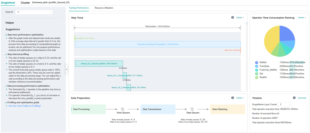
Figure:Overall Performance

Figure above displays the overall performance of the training, including the overall data of Step Trace, Operator Performance, Data Preparation Performance and Timeline. The data shown in these components include:

Step Trace: It will divide the training steps into several stages and collect execution time for each stage. The overall performance page will show the step trace graph.
Operator Performance: It will collect the execution time of operators and operator types. The overall performance page will show the pie graph for different operator types.
Data Preparation Performance: It will analyse the performance of the data input stages. The overall performance page will show the number of steps that may be the bottleneck for these stages.
Timeline: It will collect execution time for stream tasks on the devices. The tasks will be shown on the time axis. The overall performance page will show the statistics for streams and tasks.

Users can click the detail link to see the details of each components. Besides, MindSpore Insight Profiler will try to analyse the performance data, the assistant on the left will show performance tuning suggestions for this training.

Step Trace Analysis

The Step Trace Component is used to show the general performance of the stages in the training. Step Trace will divide the training into several stages:

Step Gap (The time between the end of one step and the computation of next step), Forward/Backward Propagation, All Reduce and Parameter Update. It will show the execution time for each stage, and help to find the bottleneck stage quickly.

Note

Step trace analysis only supports single-graph scenarios in Graph mode, and does not support scenarios such as pynative, heterogeneous, and multi-subgraphs.

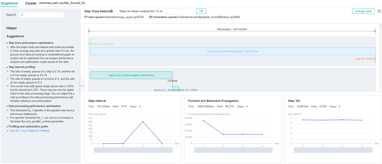
Figure:Step Trace Analysis

Figure above displays the Step Trace page. The Step Trace detail will show the start/finish time for each stage. By default, it shows the average time for all the steps. Users can also choose a specific step to see its step trace statistics.

The graphs at the bottom of the page show the execution time of Step Interval, Forward/Backward Propagation and Step Tail (The time between the end of Backward Propagation and the end of Parameter Update) changes according to different steps, it will help to decide whether we can optimize the performance of some stages. Here are more details:

Step Interval is the duration for reading data from data queues. If this part takes long time, it is advised to check the data preparation for further analysis.
Forward and Backward Propagation is the duration for executing the forward and backward operations on the network, which handle the main calculation work of a step. If this part takes long time, it is advised to check the statistics of operators or timeline for further analysis.
Step Tail is the duration for performing parameter aggregation and update operations in parallel training. If the operation takes long time, it is advised to check the statistics of communication operators and the status of parallelism.

In order to divide the stages, the Step Trace Component need to figure out the forward propagation start operator and the backward propagation end operator. MindSpore will automatically figure out the two operators to reduce the profiler configuration work. The first operator after get_next will be selected as the forward start operator and the operator before the last all reduce will be selected as the backward end operator. However, Profiler do not guarantee that the automatically selected operators will meet the user’s expectation in all cases. Users can set the two operators manually as follows:

Set environment variable PROFILING_FP_START to configure the forward start operator, for example, export PROFILING_FP_START=fp32_vars/conv2d/BatchNorm.
Set environment variable PROFILING_BP_END to configure the backward end operator, for example, export PROFILING_BP_END=loss_scale/gradients/AddN_70.

Operator Performance Analysis

The operator performance analysis component is used to display the execution time of the operators(AICORE/AICPU/HOSTCPU) during MindSpore run.

AICORE：AI Core operator is the main component of the computing core of Ascend AI processor, which is responsible for executing vector and tensor related computation intensive operators. TBE (Tensor Boost Engine) is an extended operator development tool based on TVM (Tensor Virtual Machine) framework. Users can use TBE to register AI Core operator information.
AICPU：AI CPU operator is a kind of CPU operator (including control operator, scalar, vector and other general-purpose calculations) that AI CPU is responsible for executing Hisilicon SOC in Ascend processor. The same operator in MindSpore may have AI Core operator and AI CPU operator at the same time. The framework will give priority to AI Core operator. If there is no AI Core operator or the selection is not satisfied, AI CPU operator will be called.
HOSTCPU：The host side CPU is mainly responsible for distributing the graph or operator to Ascend chip, and the operator can also be developed on the host side CPU according to the actual needs. The host CPU operator refers to the operator running on the host side CPU.

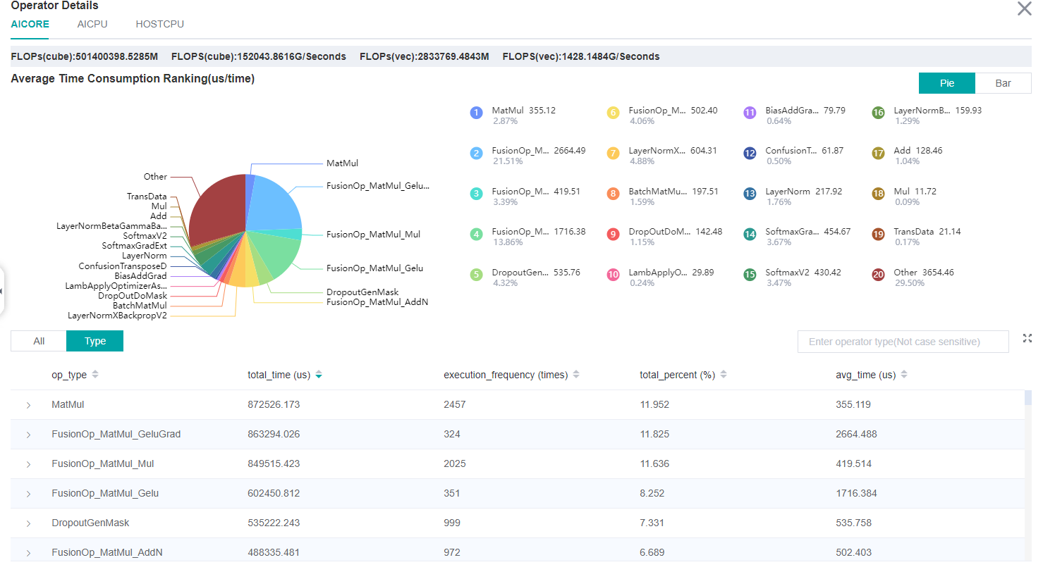
Figure:Statistics for Operator Types

Figure above displays the statistics for the operator types, including:

Choose pie or bar graph to show the proportion time occupied by each operator type. The time of one operator type is calculated by accumulating the execution time of operators belonging to this type.
Display top 20 operator types with the longest execution time, show the proportion and execution time (us) of each operator type.

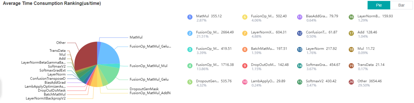
Figure:Statistics for Operators

Figure above displays the statistics table for the operators, including:

Choose All: Display statistics for the operators, including operator name, type, average execution time, execution frequency, full scope time, information, etc. The table will be sorted by execution time by default.
Choose Type: Display statistics for the operator types, including operator type name, execution time, execution frequency and proportion of total time. Users can click on each line, querying for all the operators belonging to this type.
Search: There is a search box on the right, which can support fuzzy search for operators/operator types.

Statistics for the information related to calculation quantity of AICORE operator, including operator level and model level information.

Calculation quantity analysis

The Calculation Quantity Analysis module shows the actual calculation quantity data, including calculation quantity data for operator granularity and model granularity. The actual calculation quantity refers to the amount of calculation that is running on the device, which is different from the theoretical calculation quantity. For example, the matrix computing unit on the Ascend910 device is dealing with a matrix of 16x16 size, so in the runtime, the original matrix will be padded to 16x16. Only calculation quantity on AICORE devices is supported currently. The information about calculation quantity has four indicators:

FLOPs(cube): the number of cube floating point operations (the unit is million).
FLOPS(cube): the number of cube floating point operations per second (the unit is billion).
FLOPs(vec): the number of vector floating point operations (the unit is million).
FLOPS(vec): the number of vector floating point operations per second (the unit is billion).

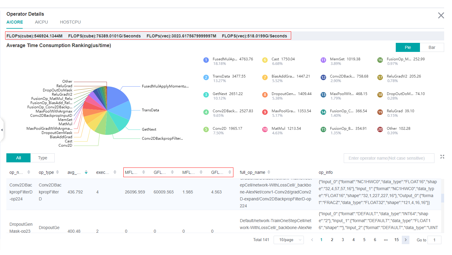
Figure:Calculation Quantity Analysis

The red box in figure above includes calculation quantity data on operator granularity and model granularity.

Data Preparation Performance Analysis

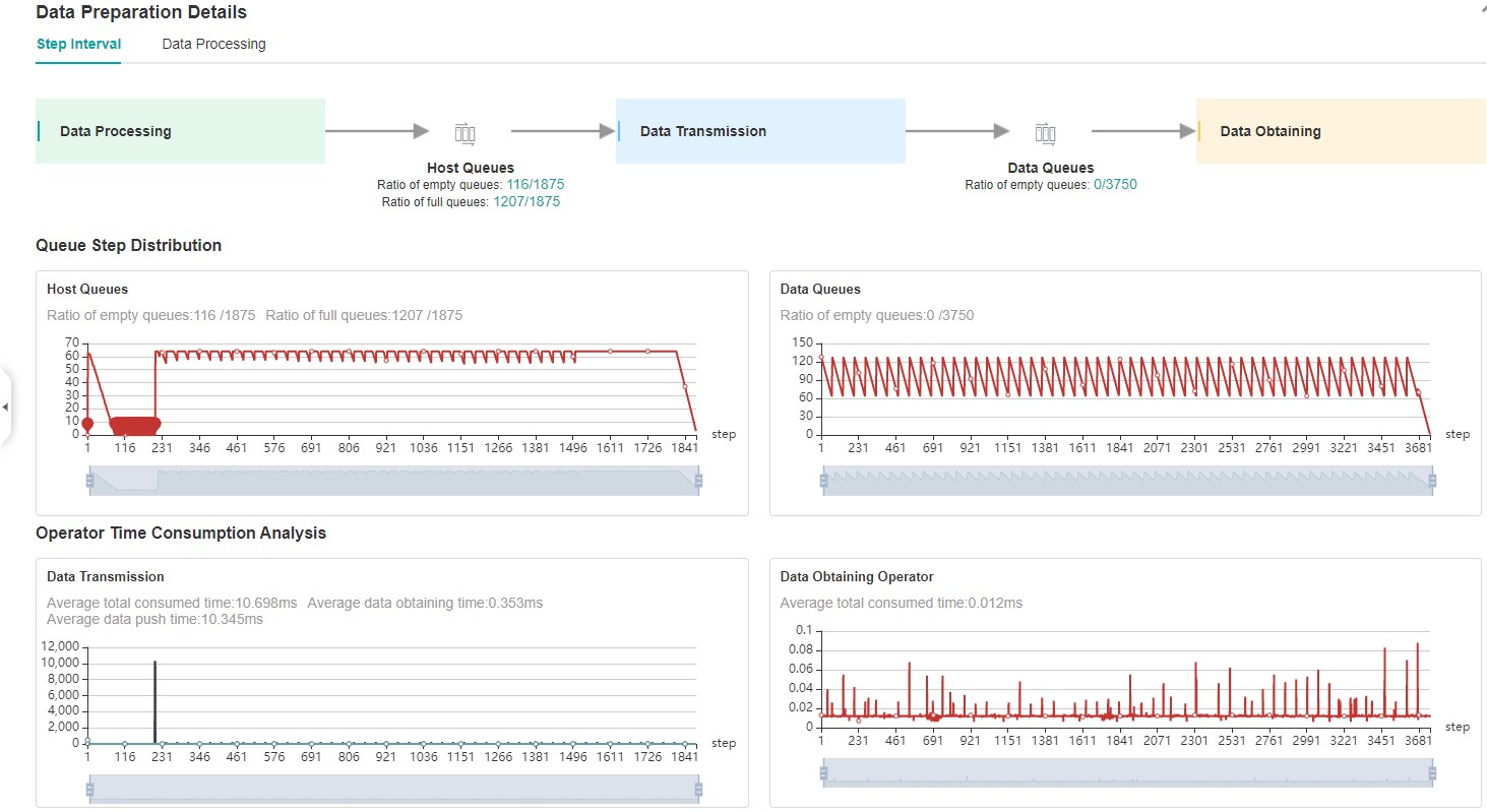
The Data preparation performance analysis component is used to analyse the execution of data input pipeline for the training. The data input pipeline can be divided into three stages:

the data process pipeline, data transfer from host to device and data fetch on device. The component will analyse the performance of each stage in detail and display the results.

Figure:Data Preparation Performance Analysis

Figure above displays the page of data preparation performance analysis component. It consists of two tabs: the step gap and the data process.

The step gap page is used to analyse whether there is performance bottleneck in the three stages. We can get our conclusion from the data queue graphs:

The data queue size stands for the queue length when the training fetches data from the queue on the device. If the data queue size is 0, the training will wait until there is data in the queue; If the data queue size is greater than 0, the training can get data very quickly, and it means data preparation stage is not the bottleneck for this training step.
The host queue size can be used to infer the speed of data process and data transfer. If the host queue size is 0, it means we need to speed up the data process stage.
If the size of the host queue is always large and the size of the data queue is continuously small, there may be a performance bottleneck in data transfer.

Note

The queue size is the value recorded when fetching data, and obtaining the data of host queue and data queue is executed asynchronously, so the number of host queue steps, data queue steps, and user training steps may be different.

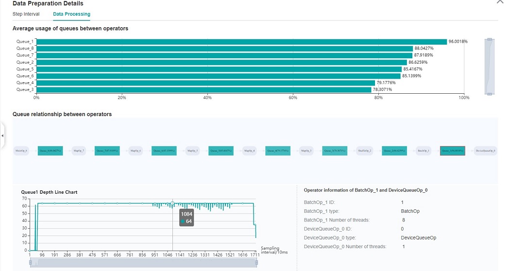
Figure:Data Process Pipeline Analysis

Figure above displays the page of data process pipeline analysis. The data queues are used to exchange data between the data processing operations. The data size of the queues reflect the data consume speed of the operations, and can be used to infer the bottleneck operation. The queue usage percentage stands for the average value of data size in queue divide data queue maximum size, the higher the usage percentage, the more data that is accumulated in the queue. The graph at the bottom of the page shows the data processing pipeline operations with the data queues, the user can click one queue to see how the data size changes according to the time, and the operations connected to the queue. The data process pipeline can be analysed as follows:

When the input queue usage percentage of one operation is high, and the output queue usage percentage is low, the operation may be the bottleneck.
For the leftmost operation, if the usage percentage of all the queues on the right are low, the operation may be the bottleneck.
For the rightmost operation, if the usage percentage of all the queues on the left are high, the operation may be the bottleneck.

To optimize the performance of data processing operations, there are some suggestions:

If the Dataset Loading Operation is the bottleneck, try to increase the num_parallel_workers.
If the GeneratorOp Operation is the bottleneck, try to increase the num_parallel_workers or try to replace it with MindRecordDataset.
If the MapOp Operation is the bottleneck, try to increase the num_parallel_workers. If it maps a Python operation, try to optimize the training script.
If the BatchOp Operation is the bottleneck, try to adjust the size of prefetch_size.

Note

To obtain data to prepare performance data, using the module of MindSpore Dataset to define data process pipeline.

Timeline Analysis

The Timeline component can display:

The operators (AICORE/AICPU/HOSTCPU operators) are executed on which device.
The MindSpore stream split strategy for this neural network.
The execution sequence and execution time of the operator on the device.
The step number of training (Currently dynamic shape scene, multi-graph scene and heterogeneous training scene are not supported, steps data may be inaccurate in these scene.).
Scope Name of the operator, the number of each operator’s Scope Name could be selected and download corresponding timeline file. For example, the full name of one operator is Default/network/lenet5/Conv2D-op11, thus the first Scope Name of this operator is Default, the second Scope Name is network. If two Scope Name for each operator is selected, then the Default and network will be displayed.

Users can get the most detailed information from the Timeline:

From the High level, users can analyse whether the stream split strategy can be optimized and whether the step tail is too long.
From the Low level, users can analyse the execution time for all the operators, etc.

Users can click the download button on the overall performance page to view Timeline details. The Timeline data file (json format) will be stored on local machine, and can be displayed by tools. We suggest to use chrome://tracing or Perfetto to visualize the Timeline.

Chrome tracing: Click “load” on the upper left to load the file.
Perfetto: Click “Open trace file” on the left to load the file.

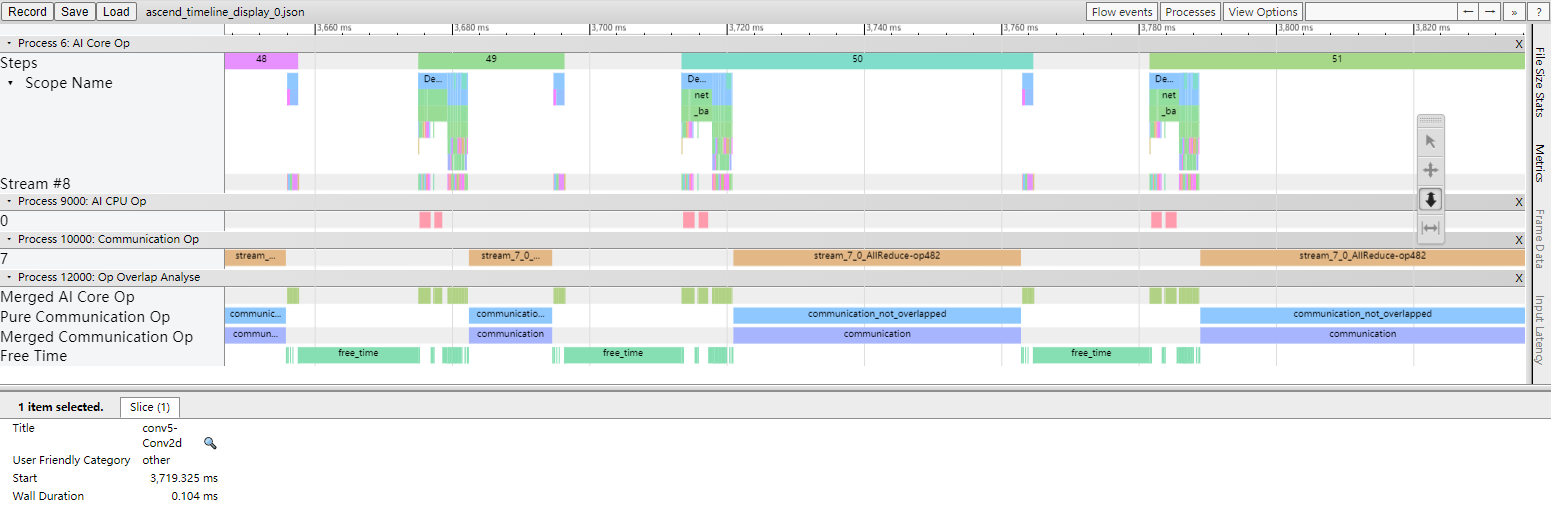
Figure:Timeline Analysis

The Timeline consists of the following parts:

Device and Stream List: It will show the stream list on each device. Each stream consists of a series of tasks. One rectangle stands for one task, and the area stands for the execution time of the task.

Each color block represents the starting time and length of operator execution. The detailed explanation of timeline is as follows:
- Process Device ID: contains the timeline of operators executed on AI Core.
  - Step: the number of training steps.
  - Scope Name: the Scope Name of operators.
  - Stream #ID: operators executed on the stream.
- Process AI CPU Op: the timeline of operators executed on the AI CPU.
- Process Communication Op: the timeline for the execution of communication operators.
- Process Host CPU Op: contains the timeline of operators executed on the Host CPU.
- Process Op Overlap Analyse: the timeline of all computation operators and communication operators merged, it can be used to analyse the proportion of communication time.
  - Merged Computation Op: it is the timeline after all computation operators are merged.
  - Merged Communication Op: it is the timeline after all communication operators are merged.
  - Pure Communication Op: pure communication time (the timeline of the communication operator after removing the overlap with the computation operator time).
  - Free Time: there is no communication operator and calculation operator in the execution timeline.
The Operator Information: When we click one task, the corresponding operator of this task will be shown at the bottom.

W/A/S/D can be applied to zoom in and out of the Timeline graph.

Timeline (Large model scenario, multi-ranks, multi-graphs, multi-iterations) Analysis

Timeline Features:

This feature is designed for the comparison and analysis of large model scenarios with multiple cards, iterations, and graphs.
Inspired by Nsight, it was first proposed to split data into two parts: summary and detail. The summary is positioned to showcase the overall execution of the model, while the detail is positioned to showcase the API level execution of the network.
The summary data include: step trace, overlap analysis of communication and computation; The detail data include: except for summary data, the execution order of calculation operators and communication operators.
Support filtering and merging data based on card number (rank id).
Support filtering and merging data based on multiple graphs (graph id).

How to view the timeline:

Click on the download button in the Timeline section of the overview page, download the timeline data(json format) locally.

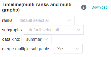
Figure：Timeline download page

As shown in the figure above:
- ranks: used for filtering and merging, default to all.
- subgraphs: used for filtering subgraphs, default to all.
- data kind: choice summary or detail, default to summary.
- merge multiple subgraphs: whether to merge the iteration trajectory data of multiple subgraphs.
Open perfetto website, drag the downloaded timeline data onto the page to complete the display.

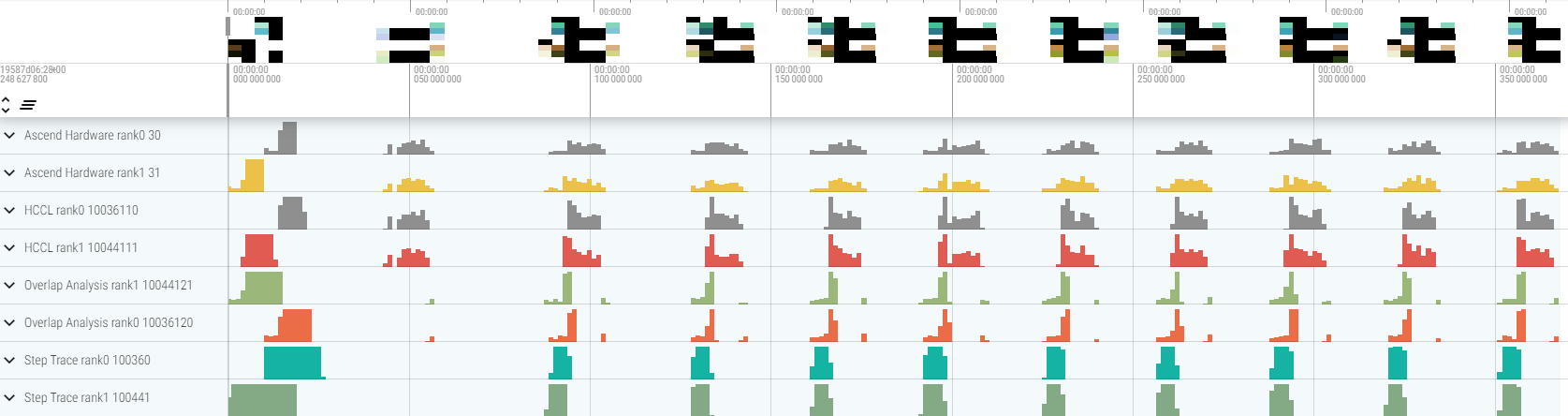
Figure：Timeline（2 ranks）Analysis

As shown in the figure above:
- Step Trace: Display the forward and backward time and iteration trailing time of each iteration according to the dimension of graph and iteration.
- Overlap Analysis: Including total network computing time, communication time, communication time not covered by computation, and card idle time.
- Ascend Hardware: Display the execution order of device side calculation operators and communication operators according to the stream.
- HCCL: Display the execution order of communication operators according to the plane.

Recommended usage of perfetto:

W/A/S/D can be applied to zoom in and out of the Timeline graph.
Select any event block, can view the detailed information of this block in the pop-up details bar below.
Mouse over multiple event blocks, can compare and analyze the execution time of multiple event blocks in the pop-up details bar below.

How to use timeline to solve practical problems：

Firstly, we recommend filtering and download summary data containing all ranks and graphs, Identify performance bottlenecks based on overall network execution to avoid premature optimization.
Then, by filtering and downloading detailed data for certain ranks and graphs, further identify performance bottlenecks at the API level and identify optimization points.
After optimizing the code, repeat the step 1 and 2 above until the performance meets the requirements.

Dynamic shape iteration analysis

When the training network is a dynamic shape network, the execution time of each operator (including AICPU operator and AICORE operator) during the operation of MindSpore can be statistically displayed by using the operator time-consuming (by iteration) component. It can quickly understand the time fluctuation of each operator in each iteration of training and the shape information of the operator in different iterations.

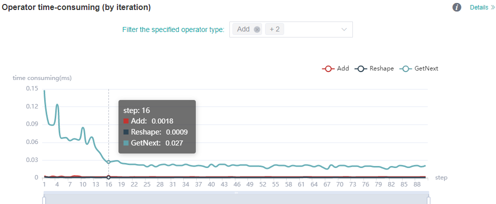
Figure: statistics of operator time (by iteration)

The figure above shows the analysis details of iteration time of different types of operators. You can view the iteration time curve of the specified operator type by filtering the specified operator type (the time shown here is the average time of the execution of different operator types).

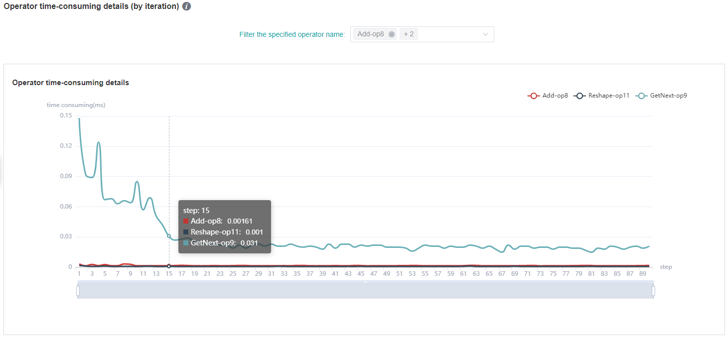
Figure: statistics of operator time-consuming details (by iteration)

The figure above shows the analysis details of iteration time of different operator instances. By filtering the specified operator name, the iteration time curve of the specified operator instance can be viewed.

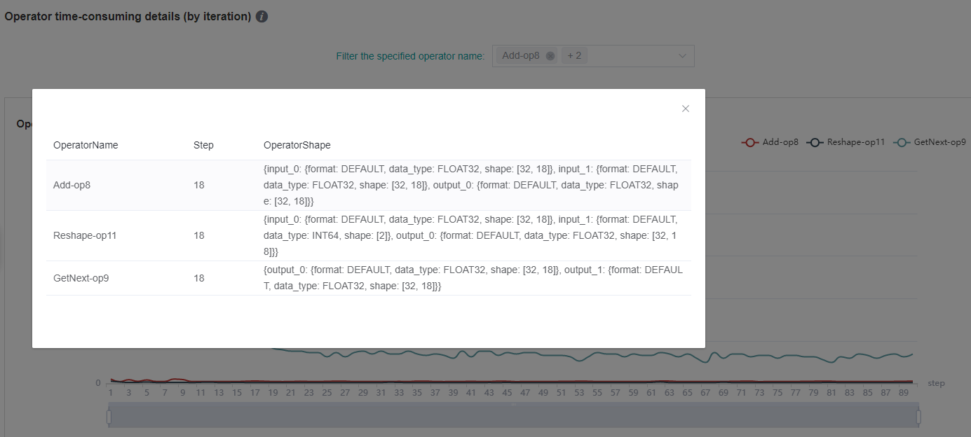
Figure: Shape information of operator (by iteration)

The figure above shows the shape information of the operator of a specific step. Click the corresponding point of the curve to check the shape information of the specified operator instance.

Note

Dynamic Shape network currently only supports the function modules of operator time (by iteration), operator time statistics ranking, data preparation, timeline, CPU utilization and parallel strategy, but does not support the functions of step trace, memory usage and cluster communication.

Msprof tool to assist analysis

Users can collect detailed data of AI Core through profiler, and then analyze and view them through Msprof tool.

The sample code is as follows:

profiler = Profiler(output_path='./data', aicore_metrics=1, l2_cache=True)

aicore_metrics is used to set the AI Core metric type, and l2_cache is used to set whether to collect l2 cache data. For parameter details, please refer to the API documentation.

MindSpore Profiler supports the collection of network performance data through the Msprof command line. For details about how to use the Msprof tool to collect and parse network performance data, please refer to the Profiling Instructions (Training) chapter of the CANN Development Tools Guide document.

Host side time consumption analysis

If the Host side time collection function is enabled, the Host side time-consuming of each stage can be saved in the specified directory after the training is completed. For example, when a Profiler is specified with output_ Path="/XXX/profiler_output" , the file containing time consumption data on the Host side will be saved in the “/XXX/profiler_output/profile/host_info” directory. The file is in json format and with the prefix "timeline_", and suffix rank_id. The host side time-consuming file can be viewed by `` chrome://tracing `` . You can use W/S/A/D to zoom in, out, move left, and right to view time consuming information.

Resource Utilization

Resource utilization includes cpu usage analysis and memory usage analysis.

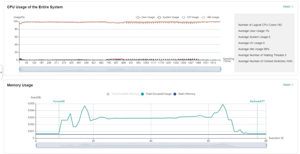
Figure:Overview of resource utilization

Overview of resource utilization：Including CPU utilization analysis and memory usage analysis. You can view the details by clicking the View Details button in the upper right corner.

CPU Utilization Analysis

CPU utilization, which is mainly used to assist performance debugging. After the performance bottleneck is determined according to the queue size, the performance can be debugged according to the CPU utilization (if the user utilization is too low, increase the number of threads; if the system utilization is too high, decrease the number of threads). CPU utilization includes CPU utilization of the whole machine, process and Data pipeline operation.

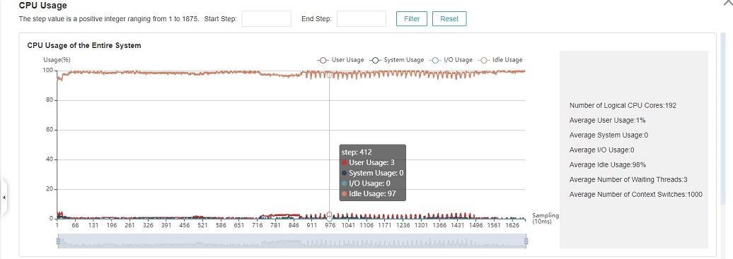
Figure:CPU utilization of the whole machine

CPU utilization of the whole machine: Show the overall CPU usage of the device in the training process, including user utilization, system utilization, idle utilization, IO utilization, current number of active processes, and context switching times. If the user utilization is low, you can try to increase the number of operation threads to increase the CPU utilization; if the system utilization is high, and the number of context switching and CPU waiting for processing is large, it indicates that the number of threads needs to be reduced accordingly.

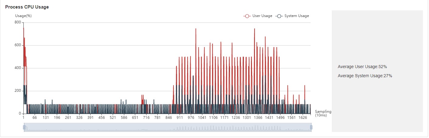
Figure:Process utilization

Process utilization: Show the CPU usage of a single process. The combination of whole machine utilization and process utilization can determine whether other processes affect the training process.

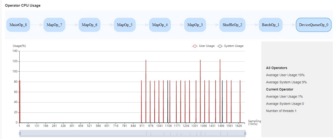
Figure:Operator utilization

Operator utilization: Show the CPU utilization of Data pipeline single operation. We can adjust the number of threads of the corresponding operation according to the actual situation. If the number of threads is small and takes up a lot of CPU, you can consider whether you need to optimize the code.

Common scenarios of CPU utilization:

According to the queue size, the network debugging personnel can judge that the performance of MindData has a bottleneck. They can adjust the number of threads by combining the utilization rate of the whole machine and the utilization rate of the operator.
Developers can check the utilization of operators. If an operation consumes CPU utilization, they can confirm whether the code needs to be optimized.

Note

The default sampling interval is 1000ms. You can change the sampling interval through mindspore.dataset.config.get_monitor_sampling_interval(). For details：

dataset API sampling interval .

Memory Analysis

This page is used to show the memory usage of the neural network model on the device, which is an ideal prediction based on the theoretical calculation results. The content of the page includes:

An overview of the memory usage of the model, including the total available memory, peak memory and other information.
The memory occupied varies in the execution order while the model is running.
The memory usage of each operator is decomposed and displayed in the table of Operator Memory Allocation.

Note

Memory Analysis does not support heterogeneous training currently.

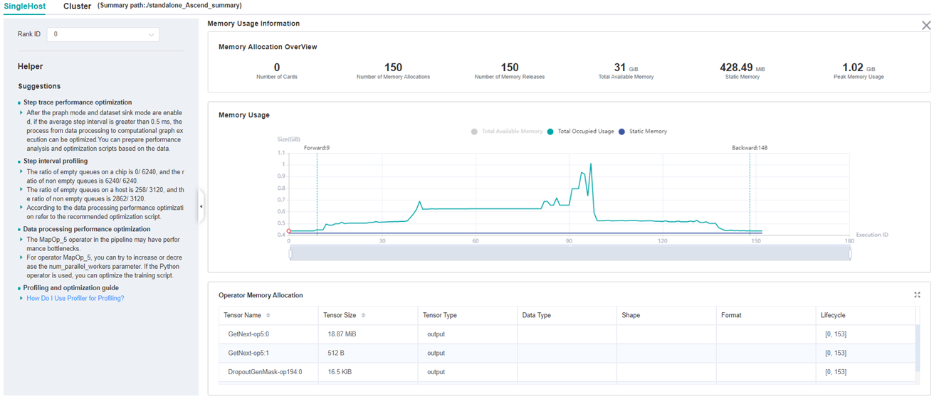
Figure:Memory Analysis

Users can obtain the summary of memory usage via the Memory Allocation Overview. In addition, they can obtain more detailed information from Memory Usage, including:

Line Chart: Changes in model memory usage, including static memory, total occupied memory and total available memory.
Zooming: There is a zoom scroll bar under the line chart. Users can zoom in or out the line chart by adjusting its size to observe more details.
FP/BP: The execution positions of the start of Forward Propagation and the end of Backward Propagation of the model on the line chart.
Details of Nodes: Hovering over the line chart, the information of the corresponding execution operator is shown, including the execution order of the operator, the name of the operator, the memory occupied by the operator, the total memory occupied by the model in the current position, and the relative memory change compared with the previous execution position.
Memory Decomposition: Left clicking a position on the line chart, the memory breakdowns of the execution position is shown in the table below the line chart, called Operator Memory Allocation. The table shows the memory decomposition of the corresponding execution position, i.e., the output tensor of which operators are allocated the occupied memory of the current execution position. The module provides users with abundant information, including tensor name, tensor size, tensor type, data type, shape, format, and the active lifetime of tensor memory.

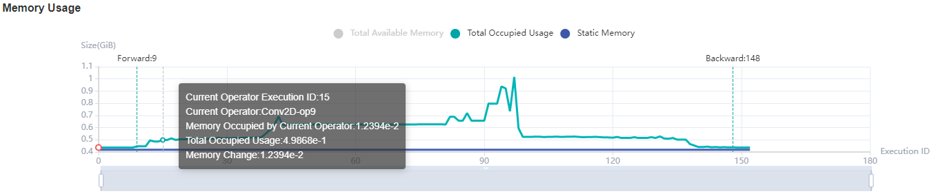
Figure:Memory Statistics

Host side memory usage

If the host side memory collection function is enabled, the memory usage can be saved in the specified directory after the training is completed. For example, when a Profiler is specified with output_ Path="/XXX/profiler_output" , the file containing host side memory data will be saved in the “/XXX/profiler_output/profile/host_info” directory. The file is in csv format and with prefix "host_memory_" and suffix rank_id. The meaning of the header is as follows:

tid: The thread ID of the current thread when collecting host side memory.
pid: The process ID of the current process when collecting host side memory.
parent_pid: The process ID of the current process’s Parent process when collecting the host side memory.
module_name: Name of the module that collects host side memory, one or more event may be included in a module.
event: The event name which collected the host side memory, one or more stage may be included in a event.
stage: The stage name which collected the host side memory.
level: 0 means used by framework developers, and 1 means used by users(algorithm engineers).
start_end: The mark for the start or end of the stage, where 0 represents the start mark, 1 represents the end mark, and 2 represents an indistinguishable start or end.
custom_info: The component customization information used by framework developers to locate performance issues, possibly empty.
memory_usage: Host-side memory usage in kB, and 0 means no memory data is collected at the current stage.
time_stamp: Time stamp in us.

Offline Analyse

When an error occurs during the training process leading to an abnormal exit, the performance file cannot be fully saved, and the Profiler provides offline parsing functionality. Currently, offline parsing only supports parsing the host side memory and host side time consumption.

For example, the partial code of the training script is as follows:

class Net(nn.Cell):
    ...


def train(net):
    ...


if __name__ == '__main__':
    ms.set_context(mode=ms.GRAPH_MODE, device_target="Ascend")

    # Init Profiler
    # Note that the Profiler should be initialized before model.train
    profiler = ms.Profiler(output_path='/path/to/profiler_data')

    # Train Model
    net = Net()
    train(net)  # Error occur.

    # Profiler end
    profiler.analyse()

If an exception occurs in above code during the training process, resulting in the profiler.analyse() at the last line not being executed, the performance data will not be completely parsed. At this point, the offline interface can be used to parse data, and the example code is as follows:

from mindspore import Profiler

profiler = Profiler(start_profile=False)
profiler.analyse(offline_path='/path/to/profiler_data')

After offline parsing, you can view the host side data in the directory /path/to/profiler_data/profile/host_info .

Specifications

To limit the data size generated by the Profiler, MindSpore Insight suggests that for large neural network, the profiled steps should be less than 10.

Note

The number of steps can be controlled by controlling the size of training dataset. For example, the num_samples parameter in mindspore.dataset.MindDataset can control the size of the dataset. For details, please refer to: dataset API .
The parse of Timeline data is time consuming, and usually the data of a few steps is enough to analyze the results. In order to speed up the data parse and UI display, Profiler will show at most 20M data (Contain 10+ step information for large networks).

Enabling the profiler has a partial performance impact on the training process. If the impact is significant, data collection items can be reduced. The following is a comparison of the performance of the Resnet network before and after enabling the profiler:

network：Resnet	Disable profiler	Enable profiler	Performance Comparison
1P+PYNATIVE	31.18444ms	31.67689ms	+0.49245ms
1P+GRAPH	30.38978ms	31.72489ms	+1.33511ms
8P+PYNATIVE	30.046ms	32.38599ms	+2.33999ms
8P+GRAPH	24.06355ms	25.04324ms	+0.97969ms

The performance data in the chart shows the average time spent on one step during the training process of the resnet network on Ascend 910. (Note: There are performance fluctuations in network training, and the above data is for reference only)

Notices

Currently the training and inference process does not support performance debugging, only individual training or inference is supported.
Step trace analysis only supports single-graph scenarios in Graph mode, and does not support scenarios such as pynative, heterogeneous, and multi-subgraphs.
Enable profiling based on step, enable profiling based on epoch, step trace analysis and cluster analysis are only supported in Graph mode.