Two-dimensional Taylor Green Vortex
![]()
![]()
![]()
This notebook requires MindSpore version >= 2.0.0 to support new APIs including: mindspore.jit, mindspore.jit_class, mindspore.jacrev.
Overview
In fluid dynamics, the Taylor–Green vortex is an unsteady flow of a decaying vortex, which has an exact closed form solution of the incompressible Navier–Stokes equations in Cartesian coordinates. It is named after the British physicist and mathematician Geoffrey Ingram Taylor and his collaborator A. E. Green.
Physics-informed Neural Networks (PINNs) provides a new method for quickly solving complex fluid problems by using loss functions that approximate governing equations coupled with simple network configurations. In this case, the data-driven characteristic of neural network is used along with PINNs to solve the 2D taylor green vortex problem
Problem Description
The Navier-Stokes equation, referred to as N-S equation, is a classical partial differential equation in the field of fluid mechanics. In the case of viscous incompressibility, the dimensionless N-S equation has the following form:
where Re stands for Reynolds number.
In this case, the PINNs method is used to learn the mapping from the location and time to flow field quantities to solve the N-S equation.
Technology Path
MindSpore Flow solves the problem as follows:
Training Dataset Construction.
Model Construction.
Multi-task Learning for Adaptive Losses
Optimizer.
NavierStokes2D.
Model Training.
Model Evaluation and Visualization.
Import necessary package
[1]:
import time
import numpy as np
import sympy
import mindspore
from mindspore import nn, ops, jit, set_seed
from mindspore import numpy as mnp
The following src pacakage can be downloaded in applications/physics_driven/taylor_green/2d/src.
[ ]:
from mindflow.cell import MultiScaleFCCell
from mindflow.utils import load_yaml_config
from mindflow.pde import NavierStokes, sympy_to_mindspore

from src import create_training_dataset, create_test_dataset, calculate_l2_error, NavierStokes2D

set_seed(123456)
np.random.seed(123456)
The following taylor_green_2D.yaml can be downloaded in applications/physics_driven/taylor_green/2d/taylor_green_2D.yaml.
[ ]:
mindspore.set_context(mode=mindspore.GRAPH_MODE, device_target="GPU", device_id=0, save_graphs=False)
use_ascend = mindspore.get_context(attr_key='device_target') == "Ascend"

config = load_yaml_config('taylor_green_2D.yaml')
Dataset Construction
Training dataset is imported through function create_train_dataset, contains domain points, initial condition points and boundary condition point. All datasets are sampled by APIs from mindflow.geometry.
Test dataset is imported through function create_test_dataset. In this case, the exact solution used to construct test dataset is given by J Kim, P Moin,Application of a fractional-step method to incompressible Navier-Stokes equations,Journal of Computational Physics,Volume 59, Issue 2,1985.
The computation is carried out in the domain of \(0 \leq x,y \leq 2\pi\), and \(0 \leq t \leq 2\). The Reynolds number Re is equal to 1
[2]:
# create training dataset
taylor_dataset = create_training_dataset(config)
train_dataset = taylor_dataset.create_dataset(batch_size=config["train_batch_size"],
                                              shuffle=True,
                                              prebatched_data=True,
                                              drop_remainder=True)

# create test dataset
inputs, label = create_test_dataset(config)
Model Construction
This example uses a simple fully-connected network with a depth of 6 layers and the activation function is the tanh function.
[3]:
coord_min = np.array(config["geometry"]["coord_min"] + [config["geometry"]["time_min"]]).astype(np.float32)
coord_max = np.array(config["geometry"]["coord_max"] + [config["geometry"]["time_max"]]).astype(np.float32)
input_center = list(0.5 * (coord_max + coord_min))
input_scale = list(2.0 / (coord_max - coord_min))

model = MultiScaleFCCell(in_channels=config["model"]["in_channels"],
                         out_channels=config["model"]["out_channels"],
                         layers=config["model"]["layers"],
                         neurons=config["model"]["neurons"],
                         residual=config["model"]["residual"],
                         act='tanh',
                         num_scales=1,
                         input_scale=input_scale,
                         input_center=input_center)
Optimizer
[4]:
params = model.trainable_params()
optimizer = nn.Adam(params, learning_rate=config["optimizer"]["initial_lr"])
Model Training
With MindSpore version >= 2.0.0, we can use the functional programming for training neural networks.
[6]:
def train():
    problem = NavierStokes2D(model, re=config["Re"])

    if use_ascend:
        from mindspore.amp import DynamicLossScaler, auto_mixed_precision, all_finite
        loss_scaler = DynamicLossScaler(1024, 2, 100)
        auto_mixed_precision(model, 'O3')

    def forward_fn(pde_data, ic_data, bc_data):
        loss = problem.get_loss(pde_data, ic_data, bc_data)
        if use_ascend:
            loss = loss_scaler.scale(loss)
        return loss

    grad_fn = mindspore.value_and_grad(forward_fn, None, optimizer.parameters, has_aux=False)

    @jit
    def train_step(pde_data, ic_data, bc_data):
        loss, grads = grad_fn(pde_data, ic_data, bc_data)
        if use_ascend:
            loss = loss_scaler.unscale(loss)
            if all_finite(grads):
                grads = loss_scaler.unscale(grads)
                loss = ops.depend(loss, optimizer(grads))
        else:
            loss = ops.depend(loss, optimizer(grads))
        return loss

    epochs = config["train_epochs"]
    steps_per_epochs = train_dataset.get_dataset_size()
    sink_process = mindspore.data_sink(train_step, train_dataset, sink_size=1)
    for epoch in range(1, 1 + epochs):
        # train
        time_beg = time.time()
        model.set_train(True)
        for _ in range(steps_per_epochs):
            step_train_loss = sink_process()
        model.set_train(False)

        if epoch % config["eval_interval_epochs"] == 0:
            print(f"epoch: {epoch} train loss: {step_train_loss} epoch time: {(time.time() - time_beg) * 1000 :.3f} ms")
            calculate_l2_error(model, inputs, label, config)
[7]:
start_time = time.time()
train()
print("End-to-End total time: {} s".format(time.time() - start_time))
momentum_x: u(x, y, t)*Derivative(u(x, y, t), x) + v(x, y, t)*Derivative(u(x, y, t), y) + Derivative(p(x, y, t), x) + Derivative(u(x, y, t), t) - 1.0*Derivative(u(x, y, t), (x, 2)) - 1.0*Derivative(u(x, y, t), (y, 2))
    Item numbers of current derivative formula nodes: 6
momentum_y: u(x, y, t)*Derivative(v(x, y, t), x) + v(x, y, t)*Derivative(v(x, y, t), y) + Derivative(p(x, y, t), y) + Derivative(v(x, y, t), t) - 1.0*Derivative(v(x, y, t), (x, 2)) - 1.0*Derivative(v(x, y, t), (y, 2))
    Item numbers of current derivative formula nodes: 6
continuty: Derivative(u(x, y, t), x) + Derivative(v(x, y, t), y)
    Item numbers of current derivative formula nodes: 2
ic_u: u(x, y, t) + sin(y)*cos(x)
    Item numbers of current derivative formula nodes: 2
ic_v: v(x, y, t) - sin(x)*cos(y)
    Item numbers of current derivative formula nodes: 2
ic_p: p(x, y, t) + 0.25*cos(2*x) + 0.25*cos(2*y)
    Item numbers of current derivative formula nodes: 3
bc_u: u(x, y, t) + exp(-2*t)*sin(y)*cos(x)
    Item numbers of current derivative formula nodes: 2
bc_v: v(x, y, t) - exp(-2*t)*sin(x)*cos(y)
    Item numbers of current derivative formula nodes: 2
bc_p: p(x, y, t) + 0.25*exp(-4*t)*cos(2*x) + 0.25*exp(-4*t)*cos(2*y)
    Item numbers of current derivative formula nodes: 3
epoch: 20 train loss: 0.11818831 epoch time: 9838.472 ms
    predict total time: 342.714786529541 ms
    l2_error, U:  0.7095809547153462 , V:  0.7081305150496081 , P:  1.004580707024092 , Total:  0.7376210740866216
==================================================================================================
epoch: 40 train loss: 0.025397364 epoch time: 9853.950 ms
    predict total time: 67.26336479187012 ms
    l2_error, U:  0.09177234501446464 , V:  0.14504987645942635 , P:  1.0217915750380309 , Total:  0.3150453016208772
==================================================================================================
epoch: 60 train loss: 0.0049396083 epoch time: 10158.307 ms
    predict total time: 121.54984474182129 ms
    l2_error, U:  0.08648064925211238 , V:  0.07875554509736878 , P:  0.711385847511365 , Total:  0.2187113170206073
==================================================================================================
epoch: 80 train loss: 0.0018874758 epoch time: 10349.795 ms
    predict total time: 85.42561531066895 ms
    l2_error, U:  0.08687053366212526 , V:  0.10624717784645109 , P:  0.3269822261697911 , Total:  0.1319986181134018
==================================================================================================
......
epoch: 460 train loss: 0.00015093417 epoch time: 9928.474 ms
    predict total time: 81.79974555969238 ms
    l2_error, U:  0.033782269766829076 , V:  0.025816595720090357 , P:  0.08782072926563861 , Total:  0.03824859644715835
==================================================================================================
epoch: 480 train loss: 6.400551e-05 epoch time: 9956.549 ms
    predict total time: 104.77519035339355 ms
    l2_error, U:  0.02242134127961232 , V:  0.021098481157660533 , P:  0.06210985820202502 , Total:  0.027418651376509482
==================================================================================================
epoch: 500 train loss: 8.7400025e-05 epoch time: 10215.720 ms
    predict total time: 77.20041275024414 ms
    l2_error, U:  0.021138056243295636 , V:  0.013343674071961624 , P:  0.045241559122240635 , Total:  0.02132725837819097
==================================================================================================
End-to-End total time: 5011.718255519867 s
Model Evaluation and Visualization
[5]:
from src import visual

# visualization
visual(model=model, epoch=config["train_epochs"], input_data=inputs, label=label)
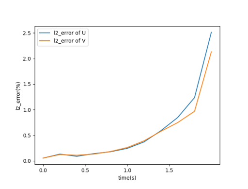
As the speed tends to decrease exponentially, the error becomes larger with time, but the overall is within the 5% error range.