Network Construction

Basic Logic

The basic logic of PyTorch and MindSpore is shown below:

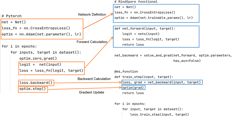
It can be seen that PyTorch and MindSpore generally require network definition, forward computation, backward computation, and gradient update steps in the implementation process.

• Network definition: In the network definition, the desired forward network, loss function, and optimizer are generally defined. To define the forward network in Net(), PyTorch network inherits from nn.Module; similarly, MindSpore network inherits from nn.Cell. In MindSpore, the loss function and optimizers can be customized in addition to using those provided in MindSpore. You can refer to Model Module Customization. Interfaces such as functional/nn can be used to splice the required forward networks, loss functions and optimizers.

• Forward computation: Run the instantiated network to get the logit, and use the logit and target as inputs to calculate the loss. It should be noted that if the forward function has more than one output, you need to pay attention to the effect of more than one output on the result when calculating the backward function.

• Backward computation: After getting the loss, we can do the backward calculation. In PyTorch the gradient can be computed using loss.backward(), and in MindSpore, the gradient can be computed by first defining the backward propagation equation net_backward using mindspore.grad(), and then passing the input into net_backward. If the forward function has more than one output, you can set has_aux to True to ensure that only the first output is involved in the derivation, and the other outputs will be returned directly in the backward calculation. For the difference in interface usage in the backward calculation, see Automatic Differentiation.

• Gradient update: Update the computed gradient into the Parameters of the network. Use optim.step() in PyTorch, while in MindSpore, pass the gradient of the Parameter into the defined optim to complete the gradient update.

Network Basic Unit: Cell

MindSpore uses Cell to construct graphs. You need to define a class that inherits the Cell base class, declare the required APIs and submodules in init, and perform calculation in construct. Cell compiles a computational graph in GRAPH_MODE (static graph mode). It is used as the basic module of neural network in PYNATIVE_MODE (dynamic graph mode).

The basic Cell setup process in PyTorch and MindSpore are as follows:

PyTorch

MindSpore

import torch.nn as torch_nn class MyCell_pt(torch_nn.Module): def __init__(self, forward_net): super(MyCell_pt, self).__init__() self.net = forward_net self.relu = torch_nn.ReLU() def forward(self, x): y = self.net(x) return self.relu(y) inner_net_pt = torch_nn.Conv2d(120, 240, kernel_size=4, bias=False) pt_net = MyCell_pt(inner_net_pt) for i in pt_net.parameters(): print(i.shape) Outputs: torch.Size([240, 120, 4, 4])

import mindspore.nn as nn import mindspore.ops as ops class MyCell(nn.Cell): def __init__(self, forward_net): super(MyCell, self).__init__(auto_prefix=True) self.net = forward_net self.relu = ops.ReLU() def construct(self, x): y = self.net(x) return self.relu(y) inner_net = nn.Conv2d(120, 240, 4, has_bias=False) my_net = MyCell(inner_net) print(my_net.trainable_params()) Outputs: [Parameter (name=net.weight, shape=(240, 120, 4, 4), dtype=Float32, requires_grad=True)]

In MindSpore, a parameter name is generally formed based on an object name defined by __init__ and a name used during parameter definition. For example, in the foregoing example, a convolutional parameter name is net.weight, where net is an object name in self.net = forward_net, and weight is name: self.weight = Parameter(initializer(self.weight_init, shape), name='weight') when a convolutional parameter is defined in Conv2d.

The cell in MindSpore provides the auto_prefix interface to determine whether to add object names to parameter names in the cell. The default value is True, that is, object names should be added. If auto_prefix is set to False, the name of Parameter printed in the preceding example is weight. In general, the backbone network should be set to True. The optimizer for training, such as :class:mindspore.nn.TrainOneStepCell, should be set to False, to avoid the parameter name in backbone be changed by mistake.

Unit Test

With the script for building the Cell, you need to use the same input data and parameters to compare the output.

import numpy as np
import mindspore as ms
import torch

x = np.random.uniform(-1, 1, (2, 120, 12, 12)).astype(np.float32)
for m in pt_net.modules():
    if isinstance(m, torch_nn.Conv2d):
        torch_nn.init.constant_(m.weight, 0.1)

for _, cell in my_net.cells_and_names():
    if isinstance(cell, nn.Conv2d):
        cell.weight.set_data(ms.common.initializer.initializer(0.1, cell.weight.shape, cell.weight.dtype))

y_ms = my_net(ms.Tensor(x))
y_pt = pt_net(torch.from_numpy(x))
diff = np.max(np.abs(y_ms.asnumpy() - y_pt.detach().numpy()))
print(diff)

# ValueError: operands could not be broadcast together with shapes (2,240,12,12) (2,240,9,9)

The output of MindSpore is different from that of PyTorch. Why?

According to the Function Differences with torch.nn.Conv2d, the default parameters of Conv2d are different in MindSpore and PyTorch. By default, MindSpore uses the same mode, and PyTorch uses the pad mode. During migration, you need to modify the pad_mode of MindSpore Conv2d.

import numpy as np
import mindspore as ms
import torch

inner_net = nn.Conv2d(120, 240, 4, has_bias=False, pad_mode="pad")
my_net = MyCell(inner_net)

# Construct random input.
x = np.random.uniform(-1, 1, (2, 120, 12, 12)).astype(np.float32)
for m in pt_net.modules():
    if isinstance(m, torch_nn.Conv2d):
        # Fixed PyTorch initialization parameter
        torch_nn.init.constant_(m.weight, 0.1)

for _, cell in my_net.cells_and_names():
    if isinstance(cell, nn.Conv2d):
        # Fixed MindSpore initialization parameter
        cell.weight.set_data(ms.common.initializer.initializer(0.1, cell.weight.shape, cell.weight.dtype))

y_ms = my_net(ms.Tensor(x))
y_pt = pt_net(torch.from_numpy(x))
diff = np.max(np.abs(y_ms.asnumpy() - y_pt.detach().numpy()))
print(diff)

Outputs:

2.9355288e-06

The overall error is about 0.01%, which basically meets the expectation. During cell migration, you are advised to perform a unit test on each cell to ensure migration consistency.

Common Methods of Cells

Cell is the basic unit of the neural network in MindSpore. It provides many easy-to-use methods. The following describes some common methods.

Manual Mixed-precision

MindSpore provides an auto mixed precision method. For details, see the amp_level attribute in Model.

However, sometimes the hybrid precision policy is expected to be more flexible during network development. MindSpore also provides the to_float method to manually add hybrid precision.

to_float(dst_type): adds type conversion to the input of the Cell and all child Cell to run with a specific floating-point type.

If dst_type is ms.float16, all inputs of Cell (including input, Parameter, and Tensor used as constants) will be converted to float16.

Customized to_float conflicts with amp_level in Model. Don't set amp_level in Model if you use custom mixed precision.

The to interface of torch.nn.Module accomplishes similar functions.

In PyTorch and MindSpore, changing all the BNs and losses in a network to be of type float32 and the rest of the operations to be of type float16 can be done:

PyTorch sets the model data type

MindSpore sets the model data type

import torch import torch.nn as nn class Network(nn.Module): def __init__(self): super(Network, self).__init__() self.layer1 = nn.Sequential( nn.Conv2d(3, 12, kernel_size=3, padding=1), nn.BatchNorm2d(12), nn.ReLU(), nn.MaxPool2d(kernel_size=2, stride=2) ) self.layer2 = nn.Sequential( nn.Conv2d(12, 4, kernel_size=3, padding=1), nn.BatchNorm2d(4), nn.ReLU(), nn.MaxPool2d(kernel_size=2, stride=2) ) self.pool = nn.AdaptiveMaxPool2d((5, 5)) self.fc = nn.Linear(100, 10) def forward(self, x): x = self.layer1(x) x = self.layer2(x) x = self.pool(x) x = x.view(x.size(0), -1) out = self.fc(x) return out net = Network() net = net.to(torch.float32) for name, module in net.named_modules(): if isinstance(module, (nn.BatchNorm1d, nn.BatchNorm2d, nn.BatchNorm3d)): module.to(torch.float32) loss = nn.CrossEntropyLoss(reduction='mean') loss = loss.to(torch.float32)

import mindspore as ms from mindspore import nn # Define model class Network(nn.Cell): def __init__(self): super().__init__() self.layer1 = nn.SequentialCell([ nn.Conv2d(3, 12, kernel_size=3, pad_mode='pad', padding=1), nn.BatchNorm2d(12), nn.ReLU(), nn.MaxPool2d(kernel_size=2, stride=2) ]) self.layer2 = nn.SequentialCell([ nn.Conv2d(12, 4, kernel_size=3, pad_mode='pad', padding=1), nn.BatchNorm2d(4), nn.ReLU(), nn.MaxPool2d(kernel_size=2, stride=2) ]) self.pool = nn.AdaptiveMaxPool2d((5, 5)) self.fc = nn.Dense(100, 10) def construct(self, x): x = self.layer1(x) x = self.layer2(x) x = self.pool(x) x = x.view((-1, 100)) out = nn.Dense(x) return out net = Network() net.to_float(ms.float16) #Add the float16 flag to all operations in the net. The framework adds the cast method to the input during compilation. for _, cell in net.cells_and_names(): if isinstance(cell, (nn.BatchNorm1d, nn.BatchNorm2d, nn.BatchNorm3d)): cell.to_float(ms.float32) loss = nn.SoftmaxCrossEntropyWithLogits(sparse=True, reduction='mean').to_float(ms.float32) net_with_loss = nn.WithLossCell(net, loss_fn=loss)

Parameters Management

In PyTorch, there are a total of four types of objects that can store data, namely Tensor, Variable, Parameter, and Buffer. The default behavior of these four objects is different. Tensor and Buffer data objects is used when the user does not require gradients, and the Variable and Parameter objects is used when the user does require gradients. PyTorch was designed to be functionally redundant (Variable will later be deprecated as well).

MindSpore optimizes the design logic of data objects by keeping only two kinds of data objects: Tensor and Parameter. The Tensor object only participates in arithmetic and does not need to perform gradient derivation and parameter update, and the Parameter data object is the same as PyTorch Parameter in the sense that its attribute requires_grad determines whether to perform gradient derivation and Parameter update. During network migration, any data object that doesn't perform Parameter update in PyTorch can be declared as a Tensor in MindSpore.

Parameter Obtaining

mindspore.nn.Cell uses the parameters_dict, get_parameters, and trainable_params interfaces to get the Parameter in Cell.

• parameters_dict: Obtain all Parameters in the network structure, and return an OrderedDict with key as the Parameter name and value as the Parameter value.

• get_parameters: Obtain all Parameters in the network structure, and return an iterator of Parameter in Cell.

• trainable_params: Obtain the attributes of Parameter where requires_grad is True, and return a list of trainable Parameters.

When defining the optimizer, use net.trainable_params() to get the list of Parameters for which Parameter updates are required.

torch.nn.Module uses the get_parameter, named_parameters, and parameters interfaces to get Parameter in Module.

PyTorch

MindSpore

import torch.nn as nn net = nn.Linear(2, 1) for name, param in net.named_parameters(): print("Parameter Name:", name) for name, param in net.named_parameters(): if "bias" in name: param.requires_grad = False for name, param in net.named_parameters(): if param.requires_grad: print("Parameter Name:", name) Outputs: Parameter Name: weight Parameter Name: bias Parameter Name: weight

import mindspore.nn as nn net = nn.Dense(2, 1, has_bias=True) print(net.trainable_params()) for param in net.trainable_params(): param_name = param.name if "bias" in param_name: param.requires_grad = False print(net.trainable_params()) Outputs: [Parameter (name=weight, shape=(1, 2), dtype=Float32, requires_grad=True), Parameter (name=bias, shape=(1,), dtype=Float32, requires_grad=True)] [Parameter (name=weight, shape=(1, 2), dtype=Float32, requires_grad=True)]

Gradient Freezing

In addition to using requires_grad=False to set the Parameter to not update the Parameter, you can also use stop_gradient to block the gradient calculation to freeze the Parameter. So when to use requires_grad=False and when to use stop_gradient?

As shown above, requires_grad=False does not update some of the Parameter, but the reverse gradient calculation is still performed normally; stop_gradient will directly truncate the reverse gradient, and the two are functionally equivalent when the frozen Parameter is not preceded by a Parameter to be trained. But stop_gradient will be faster (less part of the reverse gradient calculation is performed). Only use requires_grad=False when the frozen Parameter is preceded by a Parameter to be trained. Also, stop_gradient needs to be added to the computational link of the network, acting on the Tensor:

a = A(x)
a = ops.stop_gradient(a)
y = B(a)

Parameter Saving and Loading

MindSpore provides load_checkpoint and save_checkpoint methods for Parameter saving and loading. It should be noted that when Parameter is saved, the Parameter list is saved, and when Parameter is loaded, the object must be a Cell. When the Parameter is loaded, it is possible that the Parameter name is not correct and needs some modification, you can directly construct a new Parameter list to load_checkpoint to load into the Cell.

torch.nn.Module provides interfaces such as state_dict, load_state_dict to save and load Parameter of model.

PyTorch

MindSpore

import torch import torch.nn as nn linear_layer = nn.Linear(2, 1, bias=True) linear_layer.weight.data.fill_(1.0) linear_layer.bias.data.zero_() print("Original linear layer parameters:") print(linear_layer.weight) print(linear_layer.bias) torch.save(linear_layer.state_dict(), 'linear_layer_params.pth') new_linear_layer = nn.Linear(2, 1, bias=True) new_linear_layer.load_state_dict(torch.load('linear_layer_params.pth')) # Print the loaded Parameter, which should be the same as the original Parameter print("Loaded linear layer parameters:") print(new_linear_layer.weight) print(new_linear_layer.bias) Outputs: Original linear layer parameters: Parameter containing: tensor([[1., 1.]], requires_grad=True) Parameter containing: tensor([0.], requires_grad=True) Loaded linear layer parameters: Parameter containing: tensor([[1., 1.]], requires_grad=True) Parameter containing: tensor([0.], requires_grad=True)

import mindspore as ms import mindspore.ops as ops import mindspore.nn as nn net = nn.Dense(2, 1, has_bias=True) for param in net.get_parameters(): print(param.name, param.data.asnumpy()) ms.save_checkpoint(net, "dense.ckpt") dense_params = ms.load_checkpoint("dense.ckpt") print(dense_params) new_params = {} for param_name in dense_params: print(param_name, dense_params[param_name].data.asnumpy()) new_params[param_name] = ms.Parameter(ops.ones_like(dense_params[param_name].data), name=param_name) ms.load_param_into_net(net, new_params) for param in net.get_parameters(): print(param.name, param.data.asnumpy()) Outputs: weight [[-0.0042482 -0.00427286]] bias [0.] {'weight': Parameter (name=weight, shape=(1, 2), dtype=Float32, requires_grad=True), 'bias': Parameter (name=bias, shape=(1,), dtype=Float32, requires_grad=True)} weight [[-0.0042482 -0.00427286]] bias [0.] weight [[1. 1.]] bias [1.]

Parameter Initialization

Different Default Weight Initialization

We know that weight initialization is very important for network training. Generally, each nn interface has an implicit declaration weight. In different frameworks, the implicit declaration weight may be different. Even if the operator functions are the same, if the implicitly declared weight initialization mode distribution is different, the training process is affected or even cannot be converged.

Common nn interfaces that implicitly declare weights include Conv, Dense(Linear), Embedding, and LSTM. The Conv and Dense operators differ greatly. The Conv and Dense operators of MindSpore and PyTorch have the same distribution of weight and bias initialization methods for implicit declarations.

• Conv2d

  • mindspore.nn.Conv2d (weight: \(\mathcal{U} (-\sqrt{k},\sqrt{k} )\), bias: \(\mathcal{U} (-\sqrt{k},\sqrt{k} )\))

  • torch.nn.Conv2d (weight: \(\mathcal{U} (-\sqrt{k},\sqrt{k} )\), bias: \(\mathcal{U} (-\sqrt{k},\sqrt{k} )\))

  • tf.keras.Layers.Conv2D (weight: glorot_uniform, bias: zeros)

  In the preceding information, \(k=\frac{groups}{c_{in}*\prod_{i}^{}{kernel\_size[i]}}\)

• Dense(Linear)

  • mindspore.nn.Dense (weight: \(\mathcal{U} (-\sqrt{k},\sqrt{k} )\), bias: \(\mathcal{U} (-\sqrt{k},\sqrt{k} )\))

  • torch.nn.Linear (weight: \(\mathcal{U} (-\sqrt{k},\sqrt{k} )\), bias: \(\mathcal{U} (-\sqrt{k},\sqrt{k} )\))

  • tf.keras.Layers.Dense (weight: glorot_uniform, bias: zeros)

In the preceding information, \(k=\frac{groups}{in\_features}\).

For a network without normalization, for example, a GAN network without the BatchNorm operator, the gradient is easy to explode or disappear. Therefore, weight initialization is very important. Developers should pay attention to the impact of weight initialization.

Parameter Initializations APIs Comparison

Every API from torch.nn.init could correspond to MindSpore, except torch.nn.init.calculate_gain(). For more information, please refer to PyTorch and MindSpore API Mapping Table.

gain is used to describe the influence of the non-linearity to the standard deviation of the data. Because non-linearity will affect the standard deviation, the gradient may explode or vanish.

torch.nn.init	mindspore.common.initializer
import torch x = torch.empty(2, 2) torch.nn.init.uniform_(x)	import mindspore from mindspore.common.initializer import initializer, Uniform x = initializer(Uniform(), [1, 2, 3], mindspore.float32)

• mindspore.common.initializer is used for delayed initialization in parallel mode. Only after calling init_data(), the elements will be assigned based on its init. Every Tensor could only use init_data once. After running the code above, x is still not fully initialized. If it is used for further calculation, 0 will be used. However, when printing the Tensor, init_data() will be called automatically.

• torch.nn.init takes a Tensor as input, and the input Tensor will be changed to the target in-place. After running the code above, x is no longer an uninitialized Tensor, and its elements will follow the uniform distribution.

Customizing Initialization Parameters

Generally, the high-level API encapsulated by MindSpore initializes parameters by default. Sometimes, the initialization distribution is inconsistent with the required initialization and PyTorch initialization. In this case, you need to customize initialization. Initializing Network Arguments describes a method of initializing parameters during using API attributes. This section describes a method of initializing parameters by using Cell.

For details about the parameters, see Network Parameters. This section uses Cell as an example to describe how to obtain all parameters in Cell and how to initialize the parameters in Cell.

Note that the method described in this section cannot be performed in construct. To change the value of a parameter on the network, use assign.

For details about the parameter initialization methods supported by MindSpore, see mindspore.common.initializer. You can also directly transfer a defined Parameter object.

The created Parameter can use set_data(data, slice_shape=False) to set parameter data.

import math
import mindspore as ms
from mindspore import nn

# Define model
class Network(nn.Cell):
    def __init__(self):
        super().__init__()
        self.layer1 = nn.SequentialCell([
            nn.Conv2d(3, 12, kernel_size=3, pad_mode='pad', padding=1),
            nn.BatchNorm2d(12),
            nn.ReLU(),
            nn.MaxPool2d(kernel_size=2, stride=2)
        ])
        self.layer2 = nn.SequentialCell([
            nn.Conv2d(12, 4, kernel_size=3, pad_mode='pad', padding=1),
            nn.BatchNorm2d(4),
            nn.ReLU(),
            nn.MaxPool2d(kernel_size=2, stride=2)
        ])
        self.pool = nn.AdaptiveMaxPool2d((5, 5))
        self.fc = nn.Dense(100, 10)

    def construct(self, x):
        x = self.layer1(x)
        x = self.layer2(x)
        x = self.pool(x)
        x = x.view((-1, 100))
        out = nn.Dense(x)
        return out

net = Network()
for _, cell in net.cells_and_names():
    if isinstance(cell, nn.Conv2d):
        cell.weight.set_data(ms.common.initializer.initializer(
            ms.common.initializer.HeNormal(negative_slope=0, mode='fan_out', nonlinearity='relu'),
            cell.weight.shape, cell.weight.dtype))
    elif isinstance(cell, (nn.BatchNorm2d, nn.GroupNorm)):
        cell.gamma.set_data(ms.common.initializer.initializer("ones", cell.gamma.shape, cell.gamma.dtype))
        cell.beta.set_data(ms.common.initializer.initializer("zeros", cell.beta.shape, cell.beta.dtype))
    elif isinstance(cell, (nn.Dense)):
        cell.weight.set_data(ms.common.initializer.initializer(
            ms.common.initializer.HeUniform(negative_slope=math.sqrt(5)),
            cell.weight.shape, cell.weight.dtype))
        cell.bias.set_data(ms.common.initializer.initializer("zeros", cell.bias.shape, cell.bias.dtype))

Submodule Management

Other Cell instances may be defined as submodules in mindspore.nn.Cell. These submodules are integral parts of the network and may contain learnable Parameters (e.g., weights and biases for convolutional layers) and other submodules. This hierarchical module structure allows users to build complex and reusable neural network architectures.

mindspore.nn.Cell provides interfaces such as cells_and_names, insert_child_to_cell to realize submodule management functions.

torch.nn.Module provides interfaces such as named_modules, add_module to realize submodule management functions.

PyTorch

MindSpore

import torch.nn as nn class MyModule(nn.Module): def __init__(self): super(MyModule, self).__init__() self.conv1 = nn.Conv2d(1, 32, 3, 1) self.conv2 = nn.Conv2d(32, 64, 3, 1) # Add submodules using add_module self.add_module('conv3', nn.Conv2d(64, 128, 3, 1)) self.sequential_block = nn.Sequential( nn.ReLU(), nn.Conv2d(128, 256, 3, 1), nn.ReLU() ) def forward(self, x): x = self.conv1(x) x = self.conv2(x) x = self.conv3(x) x = self.sequential_block(x) return x module = MyModule() # Iterate through all submodules (both direct and indirect) using named_modules for name, module_instance in module.named_modules(): print(f"Module name: {name}, type: {type(module_instance)}") Output: Module name: , type: <class '__main__.MyModule'> Module name: conv1, type: <class 'torch.nn.modules.conv.Conv2d'> Module name: conv2, type: <class 'torch.nn.modules.conv.Conv2d'> Module name: conv3, type: <class 'torch.nn.modules.conv.Conv2d'> Module name: sequential_block, type: <class 'torch.nn.modules.container.Sequential'> Module name: sequential_block.0, type: <class 'torch.nn.modules.activation.ReLU'> Module name: sequential_block.1, type: <class 'torch.nn.modules.conv.Conv2d'> Module name: sequential_block.2, type: <class 'torch.nn.modules.activation.ReLU'>

from mindspore import nn class MyCell(nn.Cell): def __init__(self): super(MyCell, self).__init__() self.conv1 = nn.Conv2d(1, 32, 3, 1) self.conv2 = nn.Conv2d(32, 64, 3, 1) # Add submodules using insert_child_to_cell self.insert_child_to_cell('conv3', nn.Conv2d(64, 128, 3, 1)) self.sequential_block = nn.SequentialCell( nn.ReLU(), nn.Conv2d(128, 256, 3, 1), nn.ReLU() ) def construct(self, x): x = self.conv1(x) x = self.conv2(x) x = self.conv3(x) x = self.sequential_block(x) return x module = MyCell() # Iterate through all submodules (both direct and indirect) using cells_and_names for name, cell_instance in module.cells_and_names(): print(f"Cell name: {name}, type: {type(cell_instance)}") Output: Cell name: , type: <class '__main__.MyCell'> Cell name: conv1, type: <class 'mindspore.nn.layer.conv.Conv2d'> Cell name: conv2, type: <class 'mindspore.nn.layer.conv.Conv2d'> Cell name: conv3, type: <class 'mindspore.nn.layer.conv.Conv2d'> Cell name: sequential_block, type: <class 'mindspore.nn.layer.container.SequentialCell'> Cell name: sequential_block.0, type: <class 'mindspore.nn.layer.activation.ReLU'> Cell name: sequential_block.1, type: <class 'mindspore.nn.layer.conv.Conv2d'> Cell name: sequential_block.2, type: <class 'mindspore.nn.layer.activation.ReLU'>

Training and Evaluation Mode Switching

The torch.nn.Module provides the train(mode=True) interface to set the model in training mode and the eval interface to set the model in evaluation mode. The difference between these two modes is mainly in the behavior of layers such as Dropout and BN, as well as weight updates.

• Behavior of Dropout and BN layers:

  In training mode, the Dropout layer randomly turns off a portion of neurons according to the set Parameter p, which means that this portion of neurons will not contribute anything during the forward propagation process. The BN layer continues to compute the mean and variance and normalize the data accordingly.

  In evaluation mode, the Dropout layer does not turn off any neurons, i.e., all neurons are used for forward propagation. The BN layer uses the running mean and running variance computed during the training phase.

• Weight updates:

  In training mode, the weights of the model are updated based on the results of the backward propagation. This means that the weights of the model may change after each forward and backward propagation.

  In evaluation mode, the weights of the model are not updated. Even if forward propagation is performed and losses are computed, backpropagation is not performed to update the weights. This is because the evaluation mode is mainly used to test the performance of the model, not to train the model.

mindspore.nn.Cell provides the set_train(mode=True) interface to enable mode switching. When mode is set to True, the model is in training mode; when mode is set to False, the model is in evaluation mode.

Device Related

torch.nn.Module provides interfaces such as CPU, cuda, ipu. to move the model to the specified device.

The device_target parameter of mindspore.set_context() performs a similar function, where device_target specifies the CPU, GPU and Ascend devices. Unlike PyTorch, once the device is set, the input data and model will be copied to the specified device by default, and there is no need or possibility to change the type of device on which the data and model will be executed.

PyTorch	MindSpore
import torch torch_net = torch.nn.Linear(3, 4) torch_net.cpu()	import mindspore mindspore.set_context(device_target="CPU") ms_net = mindspore.nn.Dense(3, 4)

Dynamic and Static Graphs

For Cell, MindSpore provides two image modes: GRAPH_MODE (static image) and PYNATIVE_MODE (dynamic image). For details, see Dynamic Image and Static Graphs.

The inference behavior of the model in PyNative mode is the same as that of common Python code. However, during training, once a tensor is converted into NumPy for other operations, the gradient of the network is truncated, which is equivalent to detach of PyTorch.

When GRAPH_MODE is used, syntax restrictions usually occur. In this case, graph compilation needs to be performed on the Python code. However, MindSpore does not support the complete Python syntax set. Therefore, there are some restrictions on compiling the construct function. For details about the restrictions, see MindSpore Static Graph Syntax.

Compared with the detailed syntax description, the common restrictions are as follows:

• Scenario 1

  Restriction: During image composition (construct functions or functions modified by ms_function), do not invoke other Python libraries, such as NumPy and scipy. Related processing must be moved forward to the __init__ phase. Measure: Use the APIs provided by MindSpore to replace the functions of other Python libraries. The processing of constants can be moved forward to the __init__ phase.

• Scenario 2

  Restriction: Do not use user-defined types during graph build. Instead, use the data types provided by MindSpore and basic Python types. You can use the tuple/list combination based on these types. Measure: Use basic types for combination. You can increase the number of function parameters. There is no restriction on the input parameters of the function, and variable-length input can be used.

• Scenario 3

  Restriction: Do not perform multi-thread or multi-process processing on data during image composition. Measure: Avoid multi-thread processing on the network.

Customized Backward Network Construction

Sometimes, MindSpore does not support some processing and needs to use some third-party library methods. However, we do not want to truncate the network gradient. In this case, what should we do? This section describes how to customize backward network construction to avoid this problem in PYNATIVE_MODE.

In the following scenario, a value greater than 0.5 needs to be randomly selected, and the shape of each batch is fixed to max_num. However, the random put-back operation is not supported by MindSpore APIs. In this case, NumPy is used for computation in PYNATIVE_MODE, and then a gradient propagation process is constructed.

import numpy as np
import mindspore as ms
import mindspore.nn as nn
import mindspore.ops as ops

ms.set_context(mode=ms.PYNATIVE_MODE)
ms.set_seed(1)

class MySampler(nn.Cell):
    # Customize a sampler and select `max_num` values greater than 0.5 in each batch.
    def __init__(self, max_num):
        super(MySampler, self).__init__()
        self.max_num = max_num

    def random_positive(self, x):
        # Method of the third-party library NumPy. Select a position greater than 0.5.
        pos = np.where(x > 0.5)[0]
        pos_indice = np.random.choice(pos, self.max_num)
        return pos_indice

    def construct(self, x):
        # Forward Network Construction
        batch = x.shape[0]
        pos_value = []
        pos_indice = []
        for i in range(batch):
            a = x[i].asnumpy()
            pos_ind = self.random_positive(a)
            pos_value.append(ms.Tensor(a[pos_ind], ms.float32))
            pos_indice.append(ms.Tensor(pos_ind, ms.int32))
        pos_values = ops.stack(pos_value, axis=0)
        pos_indices = ops.stack(pos_indice, axis=0)
        print("pos_values forword", pos_values)
        print("pos_indices forword", pos_indices)
        return pos_values, pos_indices

x = ms.Tensor(np.random.uniform(0, 3, (2, 5)), ms.float32)
print("x", x)
sampler = MySampler(3)
pos_values, pos_indices = sampler(x)
grad = ms.grad(sampler, grad_position=0)(x)
print("dx", grad)

Outputs:

x [[1.2510660e+00 2.1609735e+00 3.4312444e-04 9.0699774e-01 4.4026768e-01]
 [2.7701578e-01 5.5878061e-01 1.0366821e+00 1.1903024e+00 1.6164502e+00]]
pos_values forword [[0.90699774 2.1609735  0.90699774]
 [0.5587806  1.6164502  0.5587806 ]]
pos_indices forword [[3 1 3]
 [1 4 1]]
pos_values forword [[0.90699774 1.251066   2.1609735 ]
 [1.1903024  1.1903024  0.5587806 ]]
pos_indices forword [[3 0 1]
 [3 3 1]]
dx (Tensor(shape=[2, 5], dtype=Float32, value=
[[0.00000000e+000, 0.00000000e+000, 0.00000000e+000, 0.00000000e+000, 0.00000000e+000],
 [0.00000000e+000, 0.00000000e+000, 0.00000000e+000, 0.00000000e+000, 0.00000000e+000]]),)

When we do not construct this backward process, the gradient will be truncated because the numpy method is used to calculate the pos_value. As shown in the preceding information, the value of dx is all 0s. In addition, you may find that pos_values forword and pos_indices forword are printed twice in this process. This is because the forward graph is constructed again when the backward graph is constructed in PYNATIVE_MODE. As a result, the forward graph is constructed twice and the backward graph is constructed once, which wastes training resources. In some cases, precision problems may occur. For example, in the case of BatchNorm, moving_mean and moving_var are updated during forward running. As a result, moving_mean and moving_var are updated twice during one training. To avoid this scenario, MindSpore has a method set_grad() for Cell. In PYNATIVE_MODE mode, the framework synchronously constructs the backward process when constructing the forward process. In this way, the forward process is not executed when the backward process is executed.

x = ms.Tensor(np.random.uniform(0, 3, (2, 5)), ms.float32)
print("x", x)
sampler = MySampler(3).set_grad()
pos_values, pos_indices = sampler(x)
grad = ms.grad(sampler, grad_position=0)(x)
print("dx", grad)

Outputs:

x [[1.2519144  1.6760695  0.42116082 0.59430444 2.4022336 ]
 [2.9047847  0.9402725  2.076968   2.6291676  2.68382   ]]
pos_values forword [[1.2519144 1.2519144 1.6760695]
 [2.6291676 2.076968  0.9402725]]
pos_indices forword [[0 0 1]
 [3 2 1]]
dx (Tensor(shape=[2, 5], dtype=Float32, value=
[[0.00000000e+000, 0.00000000e+000, 0.00000000e+000, 0.00000000e+000, 0.00000000e+000],
 [0.00000000e+000, 0.00000000e+000, 0.00000000e+000, 0.00000000e+000, 0.00000000e+000]]),)

Now, let's see how to customize backward network construction.

import numpy as np
import mindspore as ms
import mindspore.nn as nn
import mindspore.ops as ops

ms.set_context(mode=ms.PYNATIVE_MODE)
ms.set_seed(1)

class MySampler(nn.Cell):
    # Customize a sampler and select `max_num` values greater than 0.5 in each batch.
    def __init__(self, max_num):
        super(MySampler, self).__init__()
        self.max_num = max_num

    def random_positive(self, x):
        # Method of the third-party library NumPy. Select a position greater than 0.5.
        pos = np.where(x > 0.5)[0]
        pos_indice = np.random.choice(pos, self.max_num)
        return pos_indice

    def construct(self, x):
        # Forward network construction
        batch = x.shape[0]
        pos_value = []
        pos_indice = []
        for i in range(batch):
            a = x[i].asnumpy()
            pos_ind = self.random_positive(a)
            pos_value.append(ms.Tensor(a[pos_ind], ms.float32))
            pos_indice.append(ms.Tensor(pos_ind, ms.int32))
        pos_values = ops.stack(pos_value, axis=0)
        pos_indices = ops.stack(pos_indice, axis=0)
        print("pos_values forword", pos_values)
        print("pos_indices forword", pos_indices)
        return pos_values, pos_indices

    def bprop(self, x, out, dout):
        # Backward network construction
        pos_indices = out[1]
        print("pos_indices backward", pos_indices)
        grad_x = dout[0]
        print("grad_x backward", grad_x)
        batch = x.shape[0]
        dx = []
        for i in range(batch):
            dx.append(ops.UnsortedSegmentSum()(grad_x[i], pos_indices[i], x.shape[1]))
        return ops.stack(dx, axis=0)

x = ms.Tensor(np.random.uniform(0, 3, (2, 5)), ms.float32)
print("x", x)
sampler = MySampler(3).set_grad()
pos_values, pos_indices = sampler(x)
grad = ms.grad(sampler, grad_position=0)(x)
print("dx", grad)

Outputs:

x [[1.2510660e+00 2.1609735e+00 3.4312444e-04 9.0699774e-01 4.4026768e-01]
 [2.7701578e-01 5.5878061e-01 1.0366821e+00 1.1903024e+00 1.6164502e+00]]
pos_values forword [[0.90699774 2.1609735  0.90699774]
 [0.5587806  1.6164502  0.5587806 ]]
pos_indices forword [[3 1 3]
 [1 4 1]]
pos_indices backward [[3 1 3]
 [1 4 1]]
grad_x backward [[1. 1. 1.]
 [1. 1. 1.]]
dx (Tensor(shape=[2, 5], dtype=Float32, value=
[[0.00000000e+000, 1.00000000e+000, 0.00000000e+000, 2.00000000e+000, 0.00000000e+000],
 [0.00000000e+000, 2.00000000e+000, 0.00000000e+000, 0.00000000e+000, 1.00000000e+000]]),)

The bprop method is added to the MySampler class. The input of this method is forward input (expanded write), forward output (a tuple), and output gradient (a tuple). In this method, a gradient-to-input backward propagation process is constructed. In batch 0, the values at positions 3, 1, and 3 are randomly selected. The output gradient is 1, and the reverse gradient is [0.00000000e+000, 1.00000000e+000, 0.00000000e+000, 2.00000000e+000, 0.00000000e+000], which meets the expectation.

Random Number Strategy Comparison

Random Number APIs Comparison

There is no difference between the APIs, except that MindSpore is missing Tensor.random_, because MindSpore does not support in-place manipulations.

seed & generator

MindSpore uses seed to control the generation of a random number while PyTorch uses torch.generator.

1. There are 2 levels of random seed, graph-level and op-level. Graph-level seed is used as a global variable, and in most cases, users do not have to set the graph-level seed, they only care about the op-level seed (the parameter seed in the APIs, are all op-level seeds). If a program uses a random generator algorithm twice, the results are different even thought they are using the same seed. Nevertheless, if the user runs the script again, the same results should be obtained. For example:

   # If a random op is called twice within one program, the two results will be different:
   import mindspore as ms
   from mindspore import Tensor, ops
   
   minval = Tensor(1.0, ms.float32)
   maxval = Tensor(2.0, ms.float32)
   print(ops.uniform((1, 4), minval, maxval, seed=1))  # generates 'A1'
   print(ops.uniform((1, 4), minval, maxval, seed=1))  # generates 'A2'
   # If the same program runs again, it repeat the results:
   print(ops.uniform((1, 4), minval, maxval, seed=1))  # generates 'A1'
   print(ops.uniform((1, 4), minval, maxval, seed=1))  # generates 'A2'
   

   Different backends generate different random numbers. Here are the results from the CPU backend:

   [[1.4519546 1.242295  1.9052019 1.7309945]]
   [[1.269552  1.6567562 1.9240322 1.7505953]]
   [[1.8540323 1.3442079 1.074909  1.0930715]]
   [[1.9383929 1.8798318 1.178043  1.8124416]]
   

2. torch.Generator is often used as a key argument. A default generator will be used (torch.default_generator), when the user does not assign one to the function. torch.Generator.seed could be set with the following code:

   G = torch.Generator()
   G.manual_seed(1)
   

   It is the same as using the default generator with seed=1. e.g.: torch.manual_seed(1).

   The state of a generator in PyTorch is a Tensor of 5056 elements with dtype=uint8. When using the same generator in the script, the state of the generator will be changed. With 2 or more generators, i.e. g1 and g2, user can set g2.set_state(g1.get_state()) to make g2 have the exact same state as g1. In other words, using g2 is the same as using the g1 of that state. If g1 and g2 have the same seed and state, the random number generated by those generator are the same.